This chapter describes some experimental decoding performance figures as well as a set of limitations and considerations that have been identified for the described setup. This should be accounted for if the setup is to be utilized in a physical application.
Experimental Performance Figures
By stimulating a device with emulated quadrature pulses, the performance of the decoding scheme in terms of the maximum acceptable quadrature frequency have been explored experimentally using an ATtiny1617 running at a clock frequency of 20 MHz. These figures should be considered maximum levels for the tested device in a desktop setting with no considerable amount of noise.
For a unidirectional quadrature signal, the device could successfully count incoming pulses arriving at up to approximately 2.5 MHz. This corresponds to 75000 revolutions per minute for a rotary encoder providing 2000 counts per revolution.
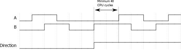
In a situation where the encoder were to oscillate in such a way that one of the input signals toggles its level continuously, corresponding to a change of direction at every edge, the interrupt routine for updating the count direction would be initiated by each of these edges. The delay associated with starting and executing the interrupt reduces the obtainable decoding frequency. The maximum acceptable frequency of consecutive direction changes was found to be approximately 500 kHz.
For comparison, a purely interrupt-based decoding scheme was also tested. The routine decides whether to count up or down for each quadrature pulse, such that the decoding is unaffected by direction changes. The maximum decoding frequency for the interrupt-based solution was found to be approximately 220 kHz.
Two advantages of a CPU-based solution compared to the core independent approach is that software filters could be implemented in order to increase noise immunity, and it adds flexibility with regards to signal processing. This would then come at the cost of a lower maximum decoding frequency.
Considerations and Limitations
The main limitations that have been identified are based on the low degree of noise immunity and the usage of interrupts for updating the count direction of the timer/counter.
Noise suppressionA low degree of internal signal filtering is used in this application in addition to edge detection on the input signals. Due to this, the decoding scheme is sensitive to noise and false spikes on the input lines. Specifically, false pulses lasting longer than one CPU clock cycle can be detected as quadrature counts or direction changes. The noise immunity will be increased by reducing the CPU clock frequency, which also reduces the decoding bandwidth accordingly. Another option is to add a level of external filtering or signal conditioning if necessary. Utilizing the index pulse signal from quadrature encoders that include this feature will reduce the functional impact if detection of false pulses can not be eliminated.
Interrupt-driven count direction updateUsing an interrupt for updating the count direction of the 16-bit Timer/Counter Type A (TCA) has some functional implications. It causes the quadrature decoding to not be fully core independent as the CPU needs to execute an interrupt routine when a direction change is detected. The CPU cycles required for handling the interrupt makes the maximum frequency of direction changes lower than the maximum frequency of quadrature pulses from unidirectional motion.