Low-Pass Filter (LPF) mode works in a similar fashion to Average mode, except that after an initial accumulation of samples, the module continues to acquire and accumulate samples indefinitely. LPF can be considered as having two main processes that work in succession - an initial average process followed by a continuous filtering operation.
The initial averaging process begins by accumulating samples until ADCNT is equal to ADRPT. During the initial process, each sample is added to the accumulator. The new accumulator value is right-shifted by the ADCRS value, and the result is loaded into ADFLTR. When ADCNT = ADRPT, a threshold test is performed on the ADFLTR value. This initial averaging process prevents threshold tests from being performed on each sample until after an average has been taken, which helps reduce ‘false alarm’ threshold violations due to random variations of a single sample. For the initial averaging process, ADRPT acts as a time constant, allowing the computed average to reach a steady state before threshold comparisons begins.
Once the initial averaging process completes, the module moves into continuous filtering operation. The module will then add the next conversion result to the accumulator to get a new accumulator value. Then, the previous accumulator value is right shifted by the ADCRS value, and then subtracted from the new accumulator value (see Figure 1).
Once these calculations have been performed, the shifted value is stored in ADFLTR as the filtered value, and a threshold test is performed. This process repeats for each new conversion. It is important to note that the accumulator is not cleared after the initial averaging process, or after any subsequent conversion, but instead continues to accumulate samples until software disables the module. During the continuous filtering operation, ADRPT is ignored, ADCNT continues to count (until ADCNT = 0xFF), and ADCRS continues to act as the accumulator divider.
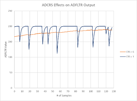
The ADCRS value also influences the filter performance. When ADCRS is a low value, the ADFLTR output reaches a steady state very quickly, but any deviations from the averaged value make a noticeable difference on the filtered output. As the ADCRS value increases, the time it takes for the ADFLTR output to achieve a steady state increases, but the effects of any deviations from the overall average have less of an impact on the filtered output (see figure below).
Table 1 shows the effects of ADCRS on the ADFLTR output. In this
comparison, the ADRES values are centered around a value of 200. At random sample points
(shaded), the ADRES values are changed to simulate an unwanted noise component that the
ADCC acquired. When the ADCRS bits are set to ‘6’, the ‘noise’ does not have much of an
effect on the filtered output. Conversely, when ADCRS is set to ‘1’,
the ‘noise’ has much more of an impact on the filtered output.
Essentially, when ADCRS values are higher, the effects of noise on the output are reduced, but sudden changes in the input may take longer to influence the output. When the ADCRS values are lower, the effects of noise have a larger impact on the filtered output, but sudden changes would be detected quickly.
Where:
ACCNEW = (ACCPREV + ADRES) -
ACCPREV = Previous accumulator result
ADRES = Current conversion result
| Sample# | ADRES | ADFLTR Output | |
|---|---|---|---|
| ADCRS = 6 | ADCRS = 1 | ||
| 0 | 200 | 166 | 198 |
| 1 | 200 | 167 | 199 |
| 2 | 200 | 167 | 199 |
| 3 | 200 | 168 | 200 |
| 7 | 100 | 168 | 150 |
| 8 | 200 | 169 | 175 |
| 17 | 200 | 173 | 200 |
| 18 | 200 | 173 | 200 |
| 19 | 50 | 171 | 125 |
| 20 | 200 | 172 | 162 |
| 36 | 200 | 178 | 200 |
| 37 | 85 | 177 | 142 |
| 38 | 200 | 177 | 171 |
| 43 | 200 | 179 | 199 |
| 44 | 85 | 177 | 142 |
| 45 | 200 | 178 | 171 |
| 55 | 200 | 181 | 200 |
| 56 | 25 | 179 | 112 |
| 82 | 200 | 186 | 200 |
| 83 | 64 | 184 | 132 |
| 128 | 200 | 188 | 196 |