| CRS | RPT | Radians @ -3dB Roll-Off |
|---|---|---|
| 1 | 2 | 0.72 |
| 2 | 4 | 0.284 |
| 3 | 8 | 0.134 |
| 4 | 16 | 0.065 |
| 5 | 32 | 0.032 |
| 6 | 64 | 0.016 |
The radian values listed in the table above are defined by the ADCC’s hardware. These values are used to calculate the -3dB roll-off point in terms of frequency. The following equation can be used to determine the -3dB point; however, there is one fundamental part of this equation that can cause confusion.
Where:
Radians @ -3dB = the value from the table above based on the CRS value
T = total sampling time
The ‘T’ term indicates the total sampling time. The total sampling time is the measured time between samples. The total sampling time is critical since it is the actual time it takes to acquire a single filtered conversion result.
The ADC’s sampling rate is only part of the total sampling time necessary to properly calculate the roll-off frequency. We know that the ADC’s sampling frequency influences the ADC result. What may not be known is that the number of instructions contained in the ADC routine also influences the total sampling time. Once the ADC’s conversion result has been acquired, the result must still pass through the filter. The conversion result may need to be sent to the DAC to output the filtered waveform, or sent to a logging file via a serial port. For example, if the ADC routine transmits the filtered result to the UART using ‘printf’ commands, the total sampling time will be longer than if the filtered value was ‘manually’ written to the UART transmit buffer. The total sampling time includes the ADC acquisition time, the conversion time, interrupt time, and any output transmission time.
The table below shows the difference in roll-off frequencies based on the sampling time ‘T’. In this example, the ADCC acquires each sample in the same manner; however, the methods used to transmit data over the UART are different. One method uses ‘printf’ statements, which are easy to use, but at the expense of additional instruction time. The other method loads the UART TX buffer with the filtered results through software instructions, which is slightly more cumbersome, but require fewer instructions than ‘printf’ statements.
- System clock (FOSC) - when used as the ADC clock, the system clock determines the TAD period
- Number of instructions - every instruction in the ADC routine takes time to execute, which adds to the total sampling time
- Number of instructions in the ISR - interrupt routines should typically be as short as possible
- Type of instructions - as previously mentioned, using the ‘printf’ library function may be very easy to use, but at the expense of additional instruction cycles
- ADC acquisition time - faster acquisition times reduce total sampling time
| CRS | Radians @ -3dB Cut-Off | Method Using ‘printf’ | Method Using Direct UART Writes | ||
|---|---|---|---|---|---|
| Measured Sampling Time (us) | Calculated Frequency @ -3dB Point (Hz) | Measured Sampling Time (us) | Calculated Frequency @ -3dB Point (Hz) | ||
| 1 | 0.72 | 520.0 | 220.37 | 435.0 | 263.43 |
| 2 | 0.284 | 520.0 | 86.92 | 435.0 | 103.91 |
| 3 | 0.134 | 520.0 | 41.01 | 435.0 | 49.03 |
| 4 | 0.065 | 520.0 | 19.89 | 435.0 | 23.78 |
| 5 | 0.032 | 520.0 | 9.79 | 435.0 | 11.71 |
| 6 | 0.016 | 520.0 | 4.90 | 435.0 | 5.85 |
One way to measure the total sampling time would be to use the Stopwatch function built in to the MPLAB® X debugger. This is accomplished by placing a breakpoint at the beginning and at the end of the ADC routine. The debugger will calculate the amount of time it takes to execute the ADC function in its entirety, including any interrupts. Of course, there are other ways to calculate the routine’s time, such as toggling a pin at the beginning and end of the routine and measuring the time in between pin states, or using a timer that is enabled at the beginning of the routine and stops at the end of the routine.
LPF EXAMPLE
This example illustrates the expected output of the ADCC using the Low-Pass
Filter function with a CRS value of ‘1’. For this example, the ‘Method
Using Direct UART Writes’ (table above) is used since it has the fastest total sampling
time, and gives a Nyquest limit of approximately 1.15 kHz.
A function generator is configured such that its output is 50 Hz sinewave, with a peak-to-peak value of 2 volts. The sinewave is offset by 1500 mV so that the voltage ranges from 500 mV to 2.5V because the ADC cannot read voltages below the negative reference voltage. The output of the function generator is connected to an analog input of the PIC18F26K42 microcontroller.
ADC Threshold interrupts are set to always interrupt after the completion of each sample.
The filtered result is copied to the UART, which sends the results to the Data Visualizer plug-in feature of the Atmel Studio 7 IDE. The Data Visualizer accepts serial data and, amongst other features, converts the data back into an analog equivalent that is shown on its built-in oscilloscope.
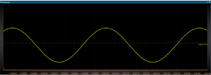
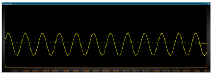
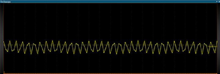
Figure 2 shows a 50 Hz sinewave reconstructed by the Data Visualizer. With the CRS value at 1, and the sample time equal to 435 μs, the 50 Hz signal is well below the expected 263 Hz roll-off point. As the sinewave’s frequency is increased, once it reaches approximately 270 Hz, a reduction in peak-to-peak voltage takes place as the filter actively reduces the magnitude of the signal, as observed in Figure 3. As the frequency continues to increase, the peak-to-peak range will shrink, as observed in Figure 4.