3 Step 3: Designing Streaming/Dataflow Hardware

The final hardware implementation covered in this tutorial is called a streaming implementation (also sometimes called a dataflow implementation). Streaming hardware can accept new inputs at a regular initiation interval (II), for example, every cycle. This bears some similarity to the loop pipelining part of the tutorial you completed above. While the streaming hardware is processing one set of inputs, new inputs can continue to be injected into the hardware every II cycles.

For example, a streaming hardware module might have a latency of 10 clock cycles and an II of 1 cycle. This would mean that, the hardware takes 10 clock cycles to complete its work for a given set of inputs. However, the hardware can continue to receive new inputs every single cycle. Streaming hardware is thus very similar to a pipelined processor, where multiple instructions are in flight at once, at intermediate stages of the pipeline. The word “streaming” is used because the generated hardware operates on a continuous stream of input data and produces a stream of output data. Image, audio, and video processing are all examples of streaming applications.

The following figure shows the 3x3 Sobel filter sweeping across an input image. From this figure, a key observation can be made. Namely, that to apply the Sobel filter, you do not need the entire input image. Instead, you only need to store the previous two rows of the input image, along with a few pixels from the current row being received (bottom row of pixels in the figure). Leveraging this observation, you can drastically reduce the amount of memory required to just two rows of the input image. The memory used to store the two rows are called “line buffers”, and they can be efficiently implemented as block RAMs on the FPGA.

1. Create a new SmartHLS project for part 3 of the tutorial and include all the .cpp and .h files for part 3. Again, specify Microsemi’s PolarFire custom device (MPF100T-FCVG484I) and finish creating the project. Examine the sobel.cpp file in the project viewer, and you will find the following line:

   static LineBuffer<unsigned char, WIDTH, 3> line_buffer;

   This statement “instantiates” SmartHLS’s LineBuffer template class from the <hls/image_processing.hpp> C++ library to create a line_buffer object. The template parameters specify the desired line buffer configuration:

   1. Use “unsigned char” 8-bit type to represent pixels
   2. Set image width to WIDTH
   3. Set the filter size to 3.

   Inside the LineBuffer, there are internal arrays for storing the previous rows (two rows when filter size is 3) and an externally accessible 2D array named window to contain pixels in the current 3x3 receptive field. The line_buffer is declared as static so that its internal state and memory are retained between functions calls.

   A few lines below, you should see line_buffer.ShiftInPixel(input_pixel);. Each call of the ShiftInPixel() function pushes in a new pixel into the line buffer and updates the line buffer’s internal previous-row arrays as well as the receptive field window. In the subsequent nested loop, you will see the 3x3 receptive field is accessed by reading the window array, i.e., line_buffer.window[m + 1][n + 1].

   A common feature of streaming hardware is called a FIFO (first-in-first-out) queue. We use FIFO queues to interconnect the various streaming components, as shown in the following figure. Here, we see a system with four streaming hardware modules, often called kernels (not to be confused with the convolutional kernels used in the Sobel filter!). The hardware kernels are connected with FIFO queues in between them. A kernel consumes data from its input FIFO queue(s) and pushes computed data into its output queue(s). If its input queue is empty, the kernel stalls (stops executing). Likewise, if the output queues are full, the unit stalls. In the example in the following figure, kernel 4 has two queues on its input, and consequently, kernel 4 commences once a data item is available in both of the queues.

   

   The SmartHLS tool provides an easy-to-use FIFO data structure to interconnect streaming kernels, which is automatically converted into a hardware FIFO during circuit synthesis. Below is a snippet from the sobel_filter function in the sobel.cpp file. Observe that the input and output FIFOs are passed by reference to the function. A pixel value is read from the input FIFO via the read() function; later, a pixel is written to the output FIFO through the write() function. These functions are declared in the hls/streaming.hpp header file.

   void sobel_filter(FIFO<unsigned char> &input_fifo,
   FIFO<unsigned char> &output_fifo) {
   ...
   unsigned char input_pixel = input_fifo.read();
   ...
   output_fifo.write(outofbounds ? 0 : sum);
   ...
   }

   The rest of the sobel_filter function is very similar to the previous parts of this tutorial. An exception relates to the use of static variables so that data can be retained across calls to the function. A count variable tracks the number of times the function has been invoked, and this is used to determine if the line buffers have been filled with data. Two static variables, i and j keep track of the row and column of the current input pixel being streamed into the function; this tracking allows the function to determine whether the pixel is out of bounds for the convolution operation (that is, on the edge of the image). The sobel_filter top-level function has an additional pragma:

   #pragma HLS function pipeline

   This pragma tells SmartHLS that the sobel_filter function is intended to be a streaming kernel.

   In the main function in sobel.cpp, you will see that FIFOs are declared in the beginning. The FIFO class has a template parameter to specify the data type stored inside the FIFO. The FIFO constructor argument specifies the depth (how many elements can be stored). In this case, the FIFOs are declared to have the unsigned char data type to create 8-bit wide FIFOs.

   In the main function, you see that the image input data (stored in input.h) is pushed into the input_fifo and the Sobel filter is invoked for HEIGHT x WIDTH times. Finally, the output values are checked for correctness and PASS or FAIL is reported. The main function returns 0 if the output values are correct.

2. Click the icons to compile
   
   and run the software
   
   , and you should see the computed and golden pixel values and the message RESULT: PASS.
3. Generate the hardware with SmartHLS by clicking on the Compile Software to Hardware icon
   
   . In the report file (summary.hls.rpt) that opens, you should see the top-level RTL interface now includes an input AXI stream interface and an output AXI stream interface, corresponding to the input_fifo and output_fifo arguments of the top-level function. Under Pipeline Result that the sobel_filter function is pipelined and has an initiation interval of 1.

   ====== 3. Pipeline Result ======
   +--------------+--------------+-------------+-------------------------+---------------------+-----------------+
   | Label | Function | Basic Block | Location in Source Code | Initiation Interval | Pipeline Length |
   +--------------+--------------+-------------+-------------------------+---------------------+-----------------+
   | sobel_filter | sobel_filter | %init.check | line 12 of sobel.cpp | 1 | 7 |
   +--------------+--------------+-------------+-------------------------+---------------------+-----------------+

   This circuit has memories inside the hardware (see Local Memories under Memory Usage) due to the line buffers and the counters that are used. You can see that there are two RAMs in the circuit, both with 4096 bits, corresponding to the two-line buffers, each storing 512 x 8-bit pixels. Note that other local memories from the report have been removed from the snippet below:

   +-----------------------------------------------------------------------------------------------------------+
   | Local Memories |
   +-----------------------------------------+-----------------------+------+-------------+------------+-------+
   | Name | Accessing Function(s) | Type | Size [Bits] | Data Width | Depth |
   +-----------------------------------------+-----------------------+------+-------------+------------+-------+
   ... ... ...
   ... ... ...
   ... ... ...
   | sobel_filter_line_buffer_prev_row_a0_a0 | sobel_filter | RAM | 4096 | 8 | 512 |
   | sobel_filter_line_buffer_prev_row_a1_a0 | sobel_filter | RAM | 4096 | 8 | 512 |

4. Simulate the streaming hardware by clicking on the SW/HW Co-Simulation icon
   
   . You will see scrolling output in the Console window, reporting the computed and expected pixel value at each clock cycle. After a few minutes, the co-simulation will finish, and in the Console, you should see:

   ...
   PASS!
   ...
   Number of calls: 262,658
   Cycle latency: 262,667
   SW/HW co-simulation: PASS

   The total number of clock cycles is about 262,667, which is very close to 512 x 512 = 262,144. The number of cycles for the streaming hardware is close to the total number of pixels computed, which confirms that you are processing 1 pixel every clock cycle (Initiation Interval is 1). At the end of the co-simulation, you should see that the co-simulation has passed.

5. You can now synthesize the circuit with Libero targeting the PolarFire FPGA by clicking on the Synthesize Hardware to FPGA icon
   
   in the toolbar. You should see the following results in the summary.results.rpt report file:

   ====== 2. Timing Result ======
   +--------------+---------------+-------------+-------------+----------+-------------+
   | Clock Domain | Target Period | Target Fmax | Worst Slack | Period | Fmax |
   +--------------+---------------+-------------+-------------+----------+-------------+
   | clk | 10.000 ns | 100.000 MHz | 6.064 ns | 3.936 ns | 254.065 MHz |
   +--------------+---------------+-------------+-------------+----------+-------------+
   ...
   ====== 3. Resource Usage ======
   +--------------------------+----------------+--------+------------+
   | Resource Type | Used | Total | Percentage |
   +--------------------------+----------------+--------+------------+
   | Fabric + Interface 4LUT* | 486 + 72 = 558 | 108600 | 0.51 |
   | Fabric + Interface DFF* | 398 + 72 = 470 | 108600 | 0.43 |
   | I/O Register | 0 | 852 | 0.00 |
   | User I/O | 0 | 284 | 0.00 |
   | uSRAM | 0 | 1008 | 0.00 |
   | LSRAM | 2 | 352 | 0.57 |
   | Math | 0 | 336 | 0.00 |
   +--------------------------+----------------+--------+------------+

   SmartHLS also allows you to give a target clock period constraint, which the compiler uses to schedule the operations in the program and insert registers so that the generated circuit can be implemented accordingly. It may not always be possible for SmartHLS to meet the user-provided target period precisely due to the complexity of the circuit or the physical properties of the target FPGA device, but in general, a lower clock period constraint leads to higher F_max. A lower clock period may cause a larger circuit area due to SmartHLS inserting more registers, and a higher clock period constraint leads to lower Fmax but can also have less area.

6. Open the HLS Constraints dialog by clicking the icon
   
   where you can change the target clock period constraint. As shown in the following figure, select Set target clock period for Constraint Type and set Constraint Value to the desired clock period in nanoseconds: 7. Click on the Add button. The constraint will appear in the list of active HLS constraints. Click on OK.

   

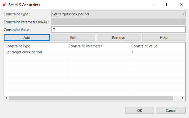
   If the target clock period constraint is not provided by you, as in this tutorial, SmartHLS will use the default target clock period constraint that has been set for each target FPGA device. The default clock period constraint is 10 ns for the Microsemi PolarFire FPGA.

7. Now that the clock period constraint is lowered to 7 ns, you can recompile software to hardware by clicking the icon
   
   . You should see the pipeline length has increased from 7 to 12 cycles as shown in the following summary.hls.rpt report file:

   ====== 3. Pipeline Result ======
   +--------------+--------------+-------------+-------------------------+---------------------+-----------------+
   | Label | Function | Basic Block | Location in Source Code | Initiation Interval | Pipeline Length |
   +--------------+--------------+-------------+-------------------------+---------------------+-----------------+
   | sobel_filter | sobel_filter | %init.check | line 12 of sobel.cpp | 1 | 12 |
   +--------------+--------------+-------------+-------------------------+---------------------+-----------------+

   The pipeline length increased because SmartHLS has added additional pipeline stages/registers to achieve the higher target Fmax. You can also synthesize the generated circuit with Libero to examine the impact of the clock period constraint on the generated circuit.