
1.3 AVR® DA Fan State Condition Monitoring Demo
Objective
Building a Machine Learning Model for Fan Condition Monitoring with MPLAB® Machine Learning Development Suite for the AVR® Curiosity Nano.
This tutorial provides a step-by-step guide on how to build a machine learning model using MPLAB® Machine Learning Development Suite for the AVR Curiosity Nano. The tutorial focuses on developing a classification model that can determine the operational state of a fan, including its on/off status, speed setting and whether it is experiencing a fault condition such as tapping, shaking or unknown issues. This tutorial includes a detailed walk-through of the Machine Learning development tools and provides high-level information on the data collection and model development process that can be applied to other applications.
Fan Condition Monitoring Project
To help users get started with their machine learning project quickly, this tutorial provides a fully developed fan condition monitoring project, including a dataset, pre-trained model, and firmware source code. This project can be utilized as a reference or starting point to built your machine learning model for Fan Condition monitoring.
Materials
Hardware Tools
Standard mounting putty, such as Loctite® Fun-Tak® mounting putty.
Any small table fan can be selected, based on personal preference. In this instance, the Honeywell HT 900 Table Fan is used as an example.
Software Tools:
MPLAB X IDE (Integrated Development Environment) (v6.05 or later)
MPLAB® Machine Learning Development Suite
ML Data Collector
ML Model Builder
Exercise Files:
The firmware and dataset used in this tutorial and other MPLAB X project files can be found in the latest GitHub release.
For more information about the IMU data collection firmware and usage instructions for Curiosity Nano, please consult the AVR DA Curiosity Nano Data Logger Github Repository.
Application Overview
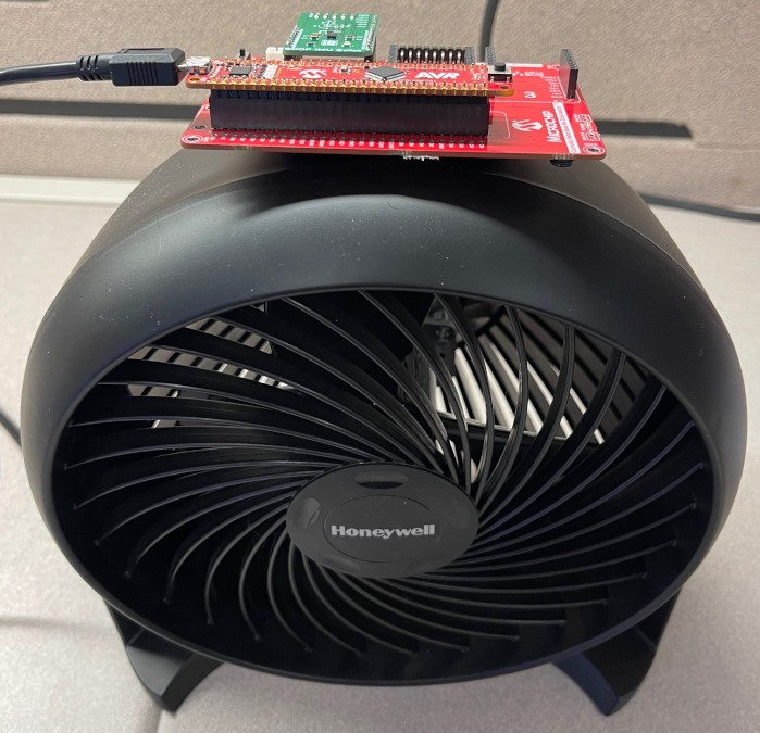
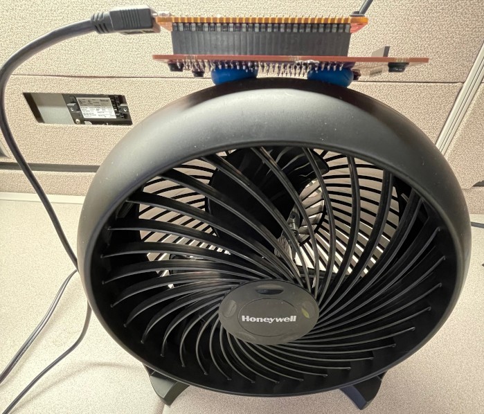
This application is focused on predictive maintenance. The objective is to evaluate whether machine learning can be utilized to monitor and predict potential machine failures, which can help reduce maintenance costs and increase uptime. The aim is to develop a classifier model using the MPLAB® Machine Learning Development Suite Toolkit that can detect the status of the fan. The model is then deployed on an AVR DA Curiosity Nano, which is installed on the fan housing. The model has the ability to differentiate between the speed modes of the fan (the HT-900 fan has three) and can also detect three abnormal states, namely tapping, shaking and unknown. The figure below shows the setup for this example application.
Data Collection Overview
In this section, the recommended approach for gathering data samples to build the fan state classifier model is discussed.
To begin the data collection process, it is essential to identify a suitable sensor configuration for your specific application. This will involve determining the optimal placement of the sensor, selecting an appropriate installation method and configuring the signal processing parameters, such as the sample rate and sensitivity.
Sensor Installation
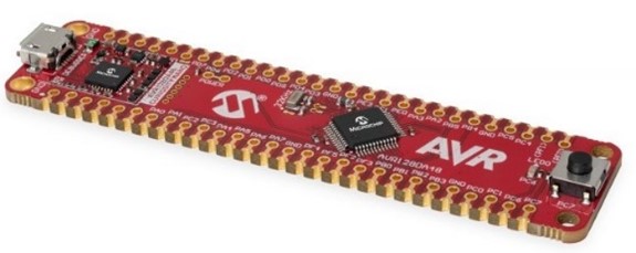
To attach the AVR DA board to the fan, a standard mounting putty was utilized, which is commonly used for mounting lightweight objects like posters onto walls. The board was placed in its default orientation, where the accelerometer reads X=0, Y=0, Z=1g. The Curiosity Nano Base board's bottom was mounted on the highest point of the fan housing. The placement was chosen for its ease of installation and no particular reason.
Sensor Sampling Configuration
The sensor sampling parameters are summarized below:
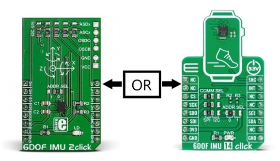
Sensor: 3-axis Accelerometer + 3-axis Gyrometer
Sample Rate / Frequency Range: 100 Hz (~40 Hz 3 dB cutoff)
Accelerometer Full Scale Range: +/-2G (most sensitive setting)
Gyrometer Full Scale Range: +/-125 DPS (most sensitive setting)
Keep in mind that the configuration above was derived from analysis on a specific fan, so it may not be optimal for different setups.
Data Collection Protocol
To proceed with the data collection process, the next essential step involves creating a protocol that outlines the necessary procedures for collecting data. This entails determining the number of samples to be collected, the metadata parameters to be captured and other relevant parameters that will govern the data collection procedure. The protocol will serve as a guide for executing the data collection process and ensure that the data collected is consistent and accurate.Data Collection: Metadata
Metadata plays a crucial role in providing context for our data. The metadata variables identified for the given application are listed and described in the table below:
Variable | Description |
Fan ID | Tag for the make, model, and serial number identifier of the fan being used |
Environment ID | Tag for the specific environment that the data was captured in |
Mount ID | Tag for the installation instance of the sensor |
Collection ID | Tag for the data collection effort where multiple samples were captured |
Data Collection: Sampling Method
At this stage, it is necessary to decide the data sampling process for our application. This involves determining the number of samples to be collected and defining the necessary steps for measuring the data. In the context of this example application, the methodology can be summarized in the following steps:
Record and label 30-second segments for each of the following fan settings: fan off, speed 1, 2 and 3.
Record tapping on the fan housing at a specific spot for a maximum of 15 seconds at a time, repeating until 30 seconds of tapping data are collected.
With the fan speed set at 1 (the slowest setting), record sensor data while gently shaking the table by grabbing either the tabletop or one of the table legs and rocking back and forth gently for a maximum of 15 seconds, repeating until 30 seconds of labeled shaking data are collected.
Executing this process once will produce enough data and variation to build a basic machine-learning model that will perform well within the experiment's constraints. However, for a more generalized model, the same collection procedure can be carried out with different fan types or by introducing realistic vibration interference that aligns with the application's conditions.
How to Configure, Compile and Flash
This document explains the steps involved in configuring the data logger firmware build, compiling it and flashing it to the AVR DA device. Follow the instructions below:-
Connect the Curiosity Nano board to your PC using a USB cable.
-
Install the MPLAB X IDE and XC8 compiler on your PC. These are essential tools for loading the data logger project and programming the AVRDA board.
-
Open the project folder
firmware/avr128da48_cnano_imu.Xin MPLAB X. -
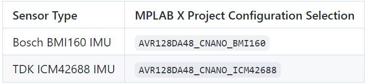
Choose the appropriate MPLAB X Project Configuration for your sensor based on the table provided below.
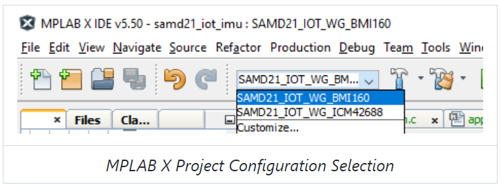
Project configuration can be set in the MPLAB X toolbar drop-down menu as shown in the image below.
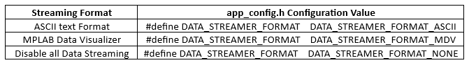
- Select the data streaming format you want
by setting the DATA_STREAMER_FORMAT macro in
firmware/src/app_config.hto the appropriate value as summarized in the table below. - Modify high-level sensor parameters like sample rate (SNSR_SAMPLE_RATE), accelerometer range (SNSR_ACCEL_RANGE) and others by changing the macro values defined in firmware/src/app_config.h. See the inline comments for further details.
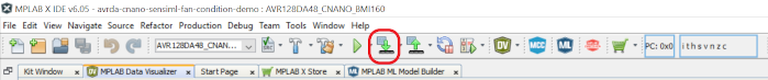
- When you are satisfied with your configuration, click the Make and Program Device icon button in the toolbar (see image below for reference).
Firmware Operation
The data streamer firmware will output sensor data over the UART port with the following UART settings:
Baud rate 115200
Data bits 8
Stop bits 1
Parity None
In addition, the on-board LED0 will indicate the firmware status as summarized in the table below:
State | LED Behaviour | Description |
Streaming | LED0 SLow Blink | Data is Streaming |
Listening | LED0 On | Waiting for connection request from MPLAB ML DCL |
Error | LED0 Off | Fatal Error (Do you have correct sensor plugged in?) |
Buffer Overflow | LED0 On for 5 seconds | Processing is not able to keep up with real-time; data Buffer was reset |
Usage with the MPLAB Data Visualizer and Machine Learning Plugins
This project can be used to generate firmware for streaming data to the MPLAB Data Visualizer plugin by setting the DATA_STREAMER_FORMAT macro to DATA_STREAMER_FORMAT_MDV as described above. When the firmware is flashed, follow the steps below to set up Data Visualizer.
Connect the Curiosity board to your computer, open up MPLAB X, then open the Data Visualizer plugin.
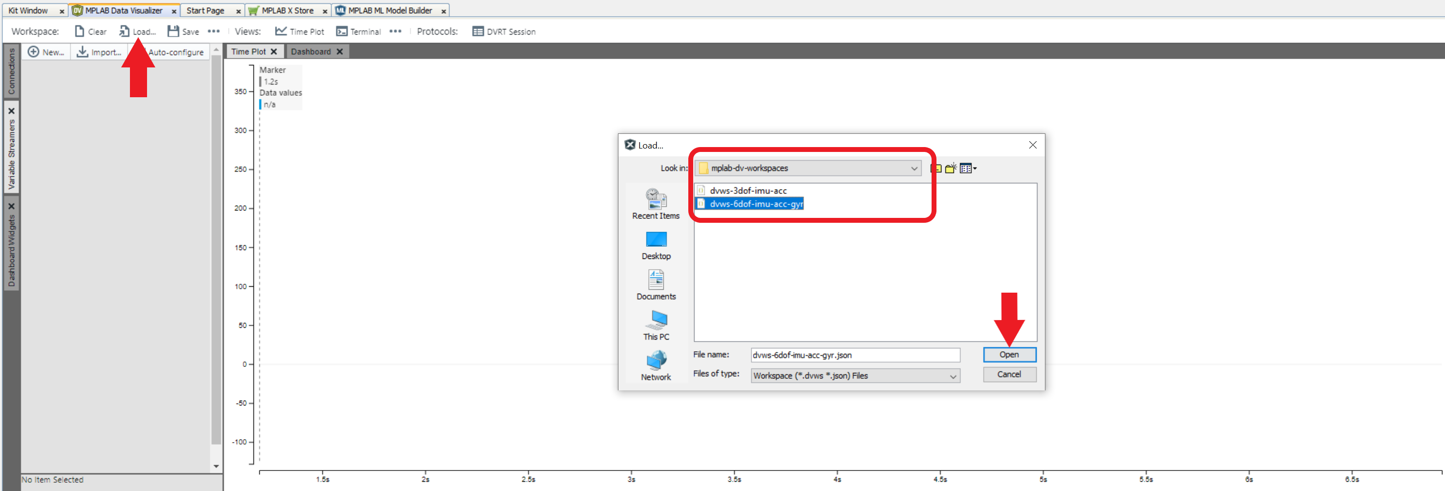
Click the Load Workspace button as highlighted in the image below. Select one of the workspace files included in this repository - located under the mplab-dv-workspaces folder - whose name most closely describes your sensor configuration; you can always modify the configuration when it is loaded if needed.
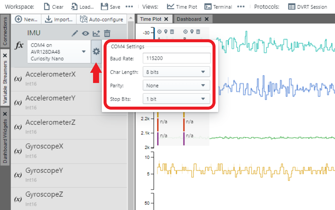
Next, select the Serial/CDC Connection that corresponds to the Curiosity board, adjust the baud rate to 115200, then click Apply.
Use the play button on the Serial/CDC Connection to connect to the serial port. When the connection is made, the AVRDA is available for use with the variable streamer.
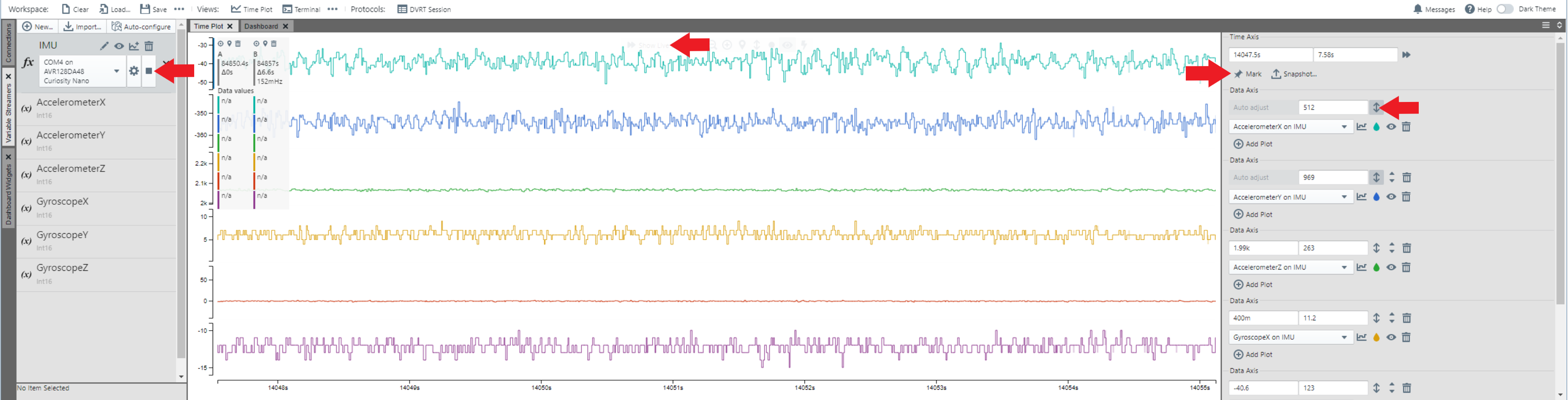
Switch to the Variable Streamers tab, then select the aforementioned Serial/CDC Connection from the dropdown menu as the input data source for the IMU variable streamer (see image below for reference); this will enable parsing of the AVRDA data stream. You may delete or add variables here if your sensor configuration differs from the pre-loaded ones.
The IMU data is now available in the time plot. Double click anywhere within the time plot to start/stop scrolling of the time axis.
Click the up down arrow button to auto set the time scale.
Click the mark icon button, then the snapshot icon button to snip the part of the time plot as data to save.
Visit the Machine Learning Plugin page to learn more about using the Data Visualizer plugin to export your data for machine learning applications.
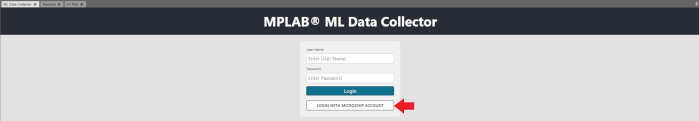
Next, open the MPLAB ML Data Collector Tool, then log in using your Microchip account. In some instances, users might see a popup where they are required to click 'Accept Cookies' to proceed.
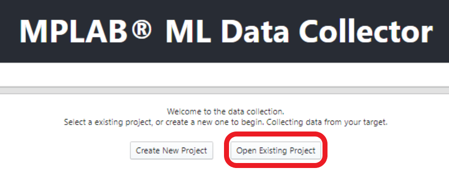
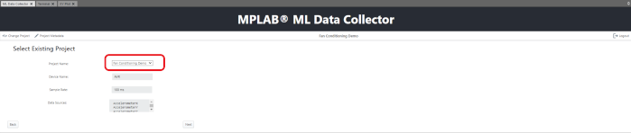
Click Open Existing Project, then choose the project that you are working on.
When done in both windows [MPLAB Data Visualizer and MPLAB ML Data Collector], they will display in parallel. For the next step:
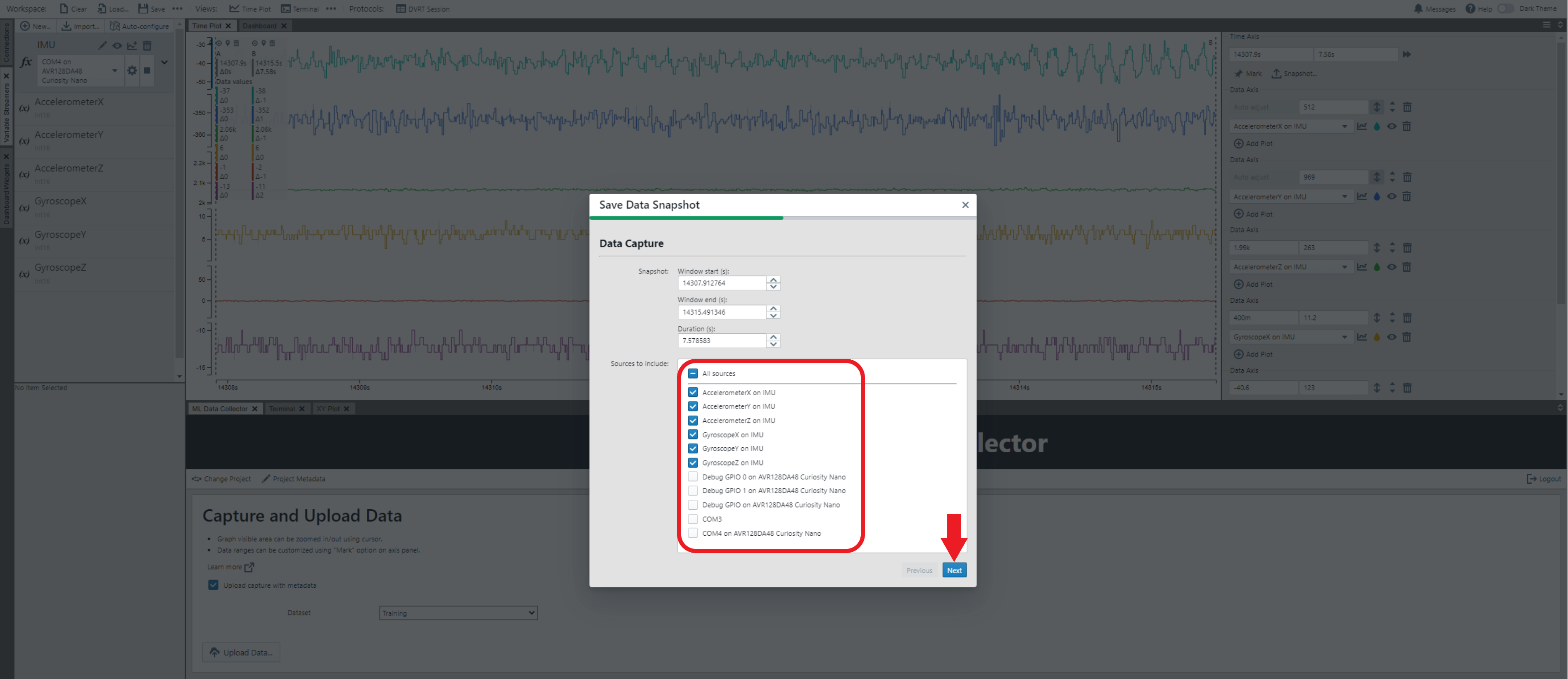
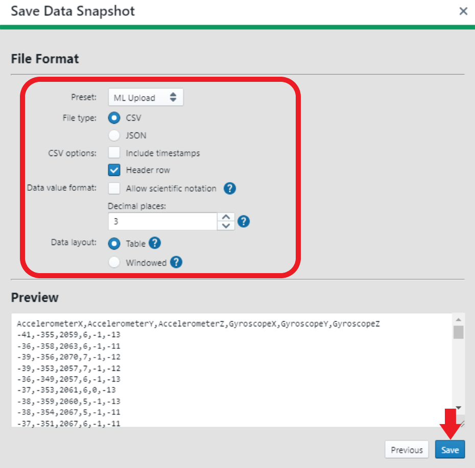
Click the snapshot icon button located on the toolbar of MPLAB Data Visualizer.
A pop-up window will appear as shown in the image below.
Set the parameters according to your preferences.
Click the Next button to proceed.
Model Development
Assuming that you have gathered an initial dataset for your application, the next step is to proceed to the ML Model Builder to create your classifier model. To generate your classifier model, proceed to MPLAB Machine Learning Development Suite.
The process for accessing the Microchip MPLAB Machine Learning Development Suite requires the following steps:
Launch the MPLAB X IDE software.
Next, launch the ML Model Builder tool.
When the ML Model Builder page loads, you will be prompted to authenticate your account by entering your myMicrochip login credentials.
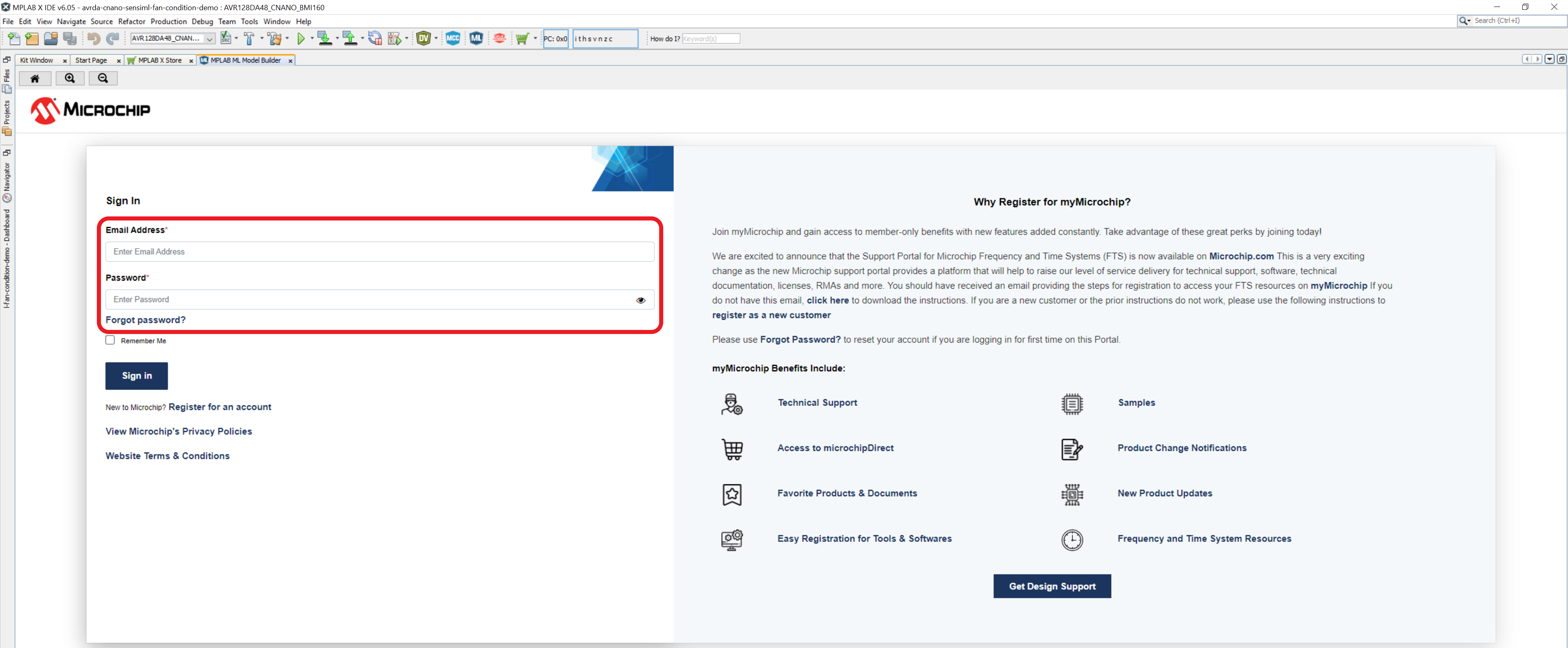
In some instances, users might see a popup where they are required to click 'Accept Cookies' to proceed.
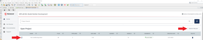
Upon successful login, you may proceed to initiate a new project by selecting the CREATE PROJECT tab. This action will trigger a pop-up window prompting you to specify a name for the new project.
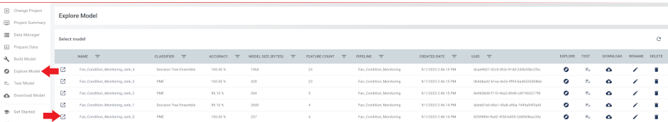
To open the project, locate the Open Project icon button located before the project name, then click it.
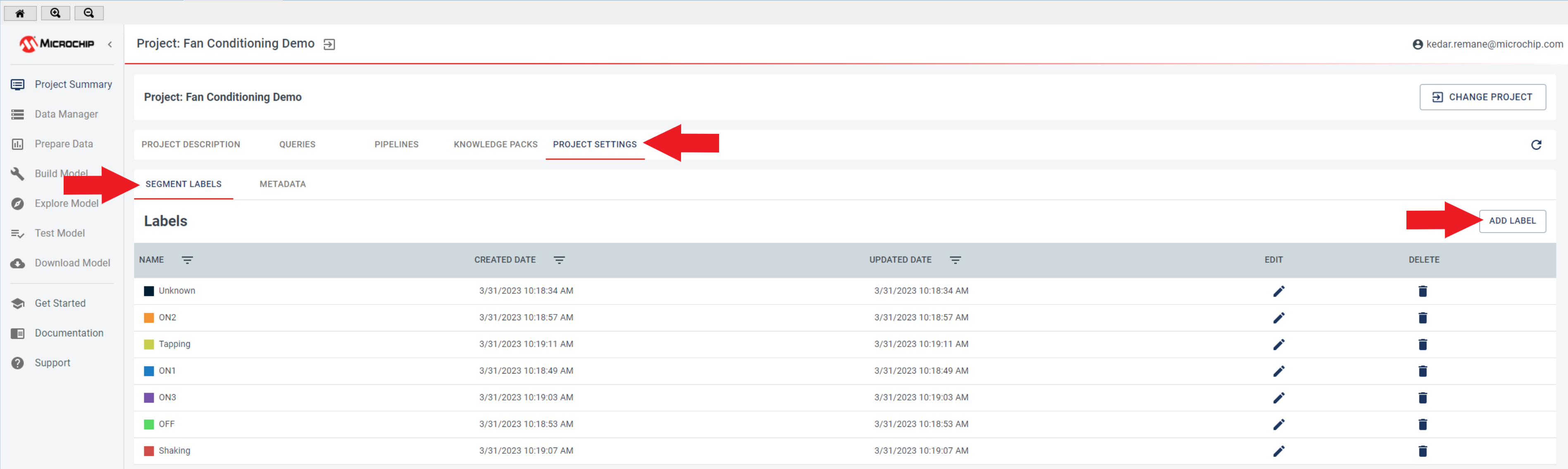
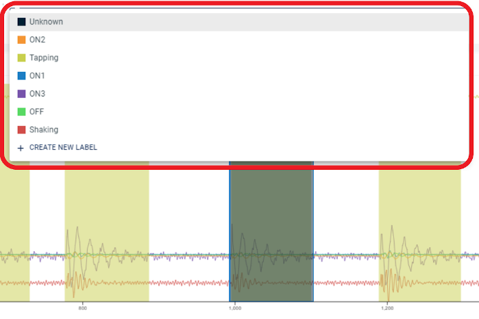
To create new labels and metadata fields for a project, follow these steps:
Go to the Project Summary page.
Click Project Settings.
You will see two fields: “Segment Labels” and “Metadata”.
To create new labels and metadata fields, click the Add Label and Add Metadata tabs located in the top right corner of the page.
Fill in the required information for the new label and metadata fields.
Click Save to create the new label and metadata field.
Repeat steps 4-6 for each additional label or metadata field that you want to create.
Next, to import necessary data files for the project, follow these steps:
Navigate to the Data Manager tab.
Locate the IMPORT CAPTURE FILE button, then click it.
Ensure that the data files to be imported are in either CSV or Wav format.
Select all the files required for the project.
Begin the import process.
When the import process is complete, the imported data files will be available for use in the project. It is important to ensure that all data files are properly formatted and labeled to ensure accurate analysis and interpretation of the project results.
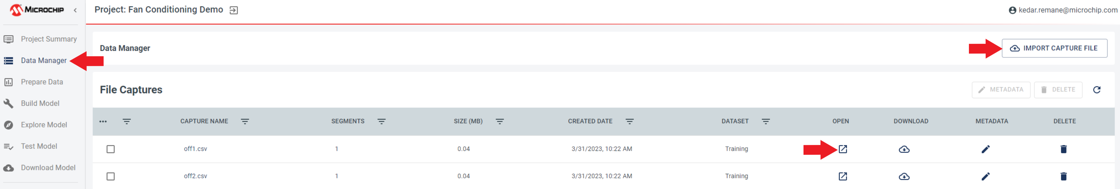
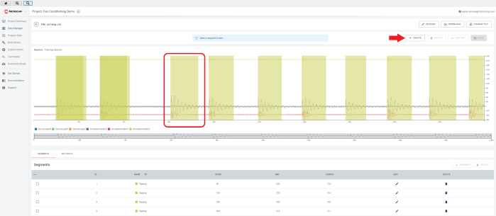
To access the imported data files, click the icons corresponding to the desired file under the OPEN column. Once the desired file is open, navigate to the CREATE tab to begin segmenting the data. To create segments, drag the segments axis to the desired locations within the data. It is, then, recommended to correctly categorize these segments using appropriate labels and metadata fields for ease of organization and future analysis.
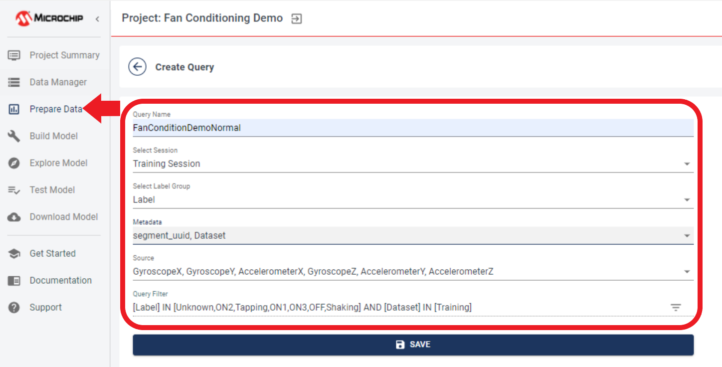
To proceed, navigate to the Prepare Data view. From there, locate and click the CREATE QUERY button to initiate the data preparation process.
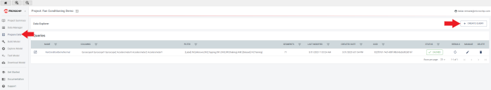
Fill out the block as displayed below.
Press the CACHE button to initiate the caching process.
Wait for the cache to build out completely.
Click the SAVE button when the cache is fully built.
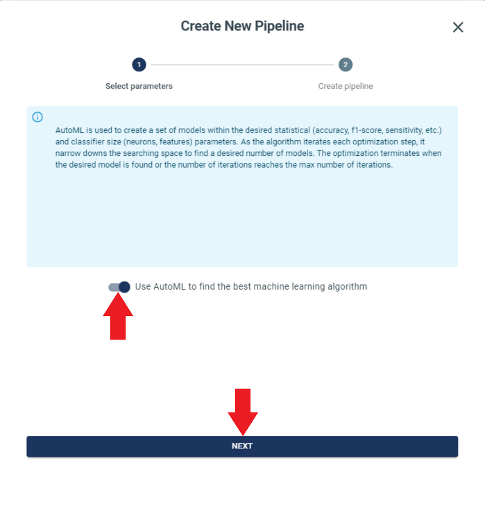
To proceed with building the pipeline, navigate to the Build Model view, then locate the Create Pipeline module.
After clicking CREATE NEW PIPELINE, information regarding AutoML displays. Make sure the “Use AutoML to find the best machine learning algorithm” is enabled. Click NEXT when finished.
Here, you need to select the query that you want to use for building the pipeline. In the example below, FanConditionDemoNormal is selected as the query and named Pipeline as FanConditionDemoPipelineN. When you have selected the query, be sure to click the CREATE PIPELINE button to save your selection.
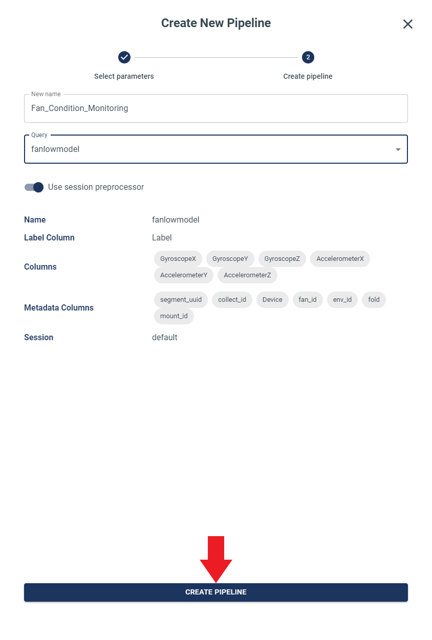
Click the First Module named Type: Input Query, then, make sure that the correct Query is selected for proceeding with the optimization.
The pipeline will be created showing parameters that will be used while building the Model. Click NEXT.
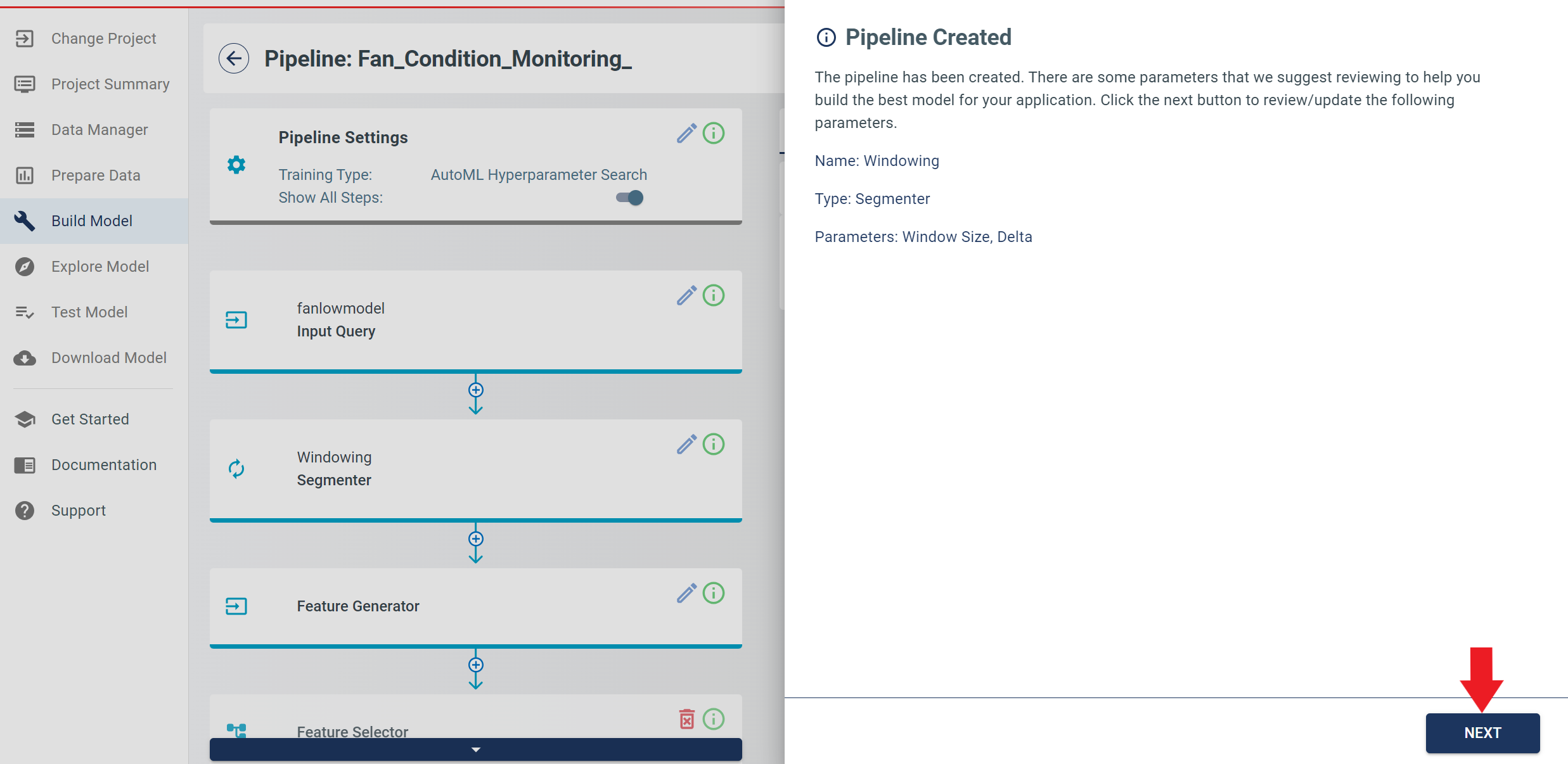
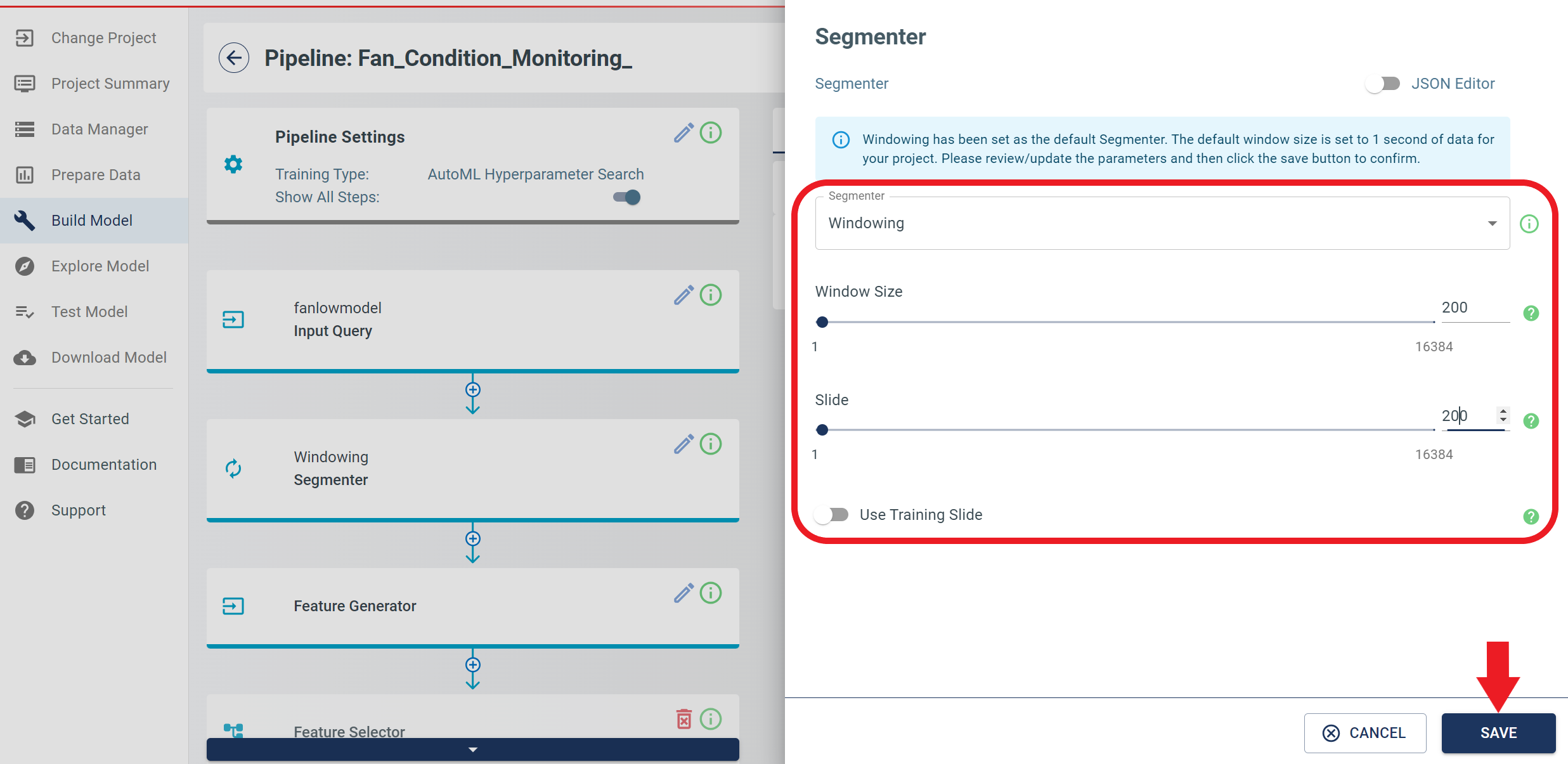
The next window is the Segmenter module, which performs segmentation of the data. Set the parameters as depicted in the figure below to ensure the appropriate segmentation of the data. After setting the parameters, click the SAVE button to save the changes made.
To proceed with the configuration process, navigate to the Pipeline Settings tab. Verify that all parameters are configured according to the parameters shown in the figure below. Click the SAVE button to save your settings.
The AutoML techniques will automatically select the best features and machine learning algorithm for the gesture classification task based on the input data you provided. Note that this optimization process typically takes several minutes to complete.
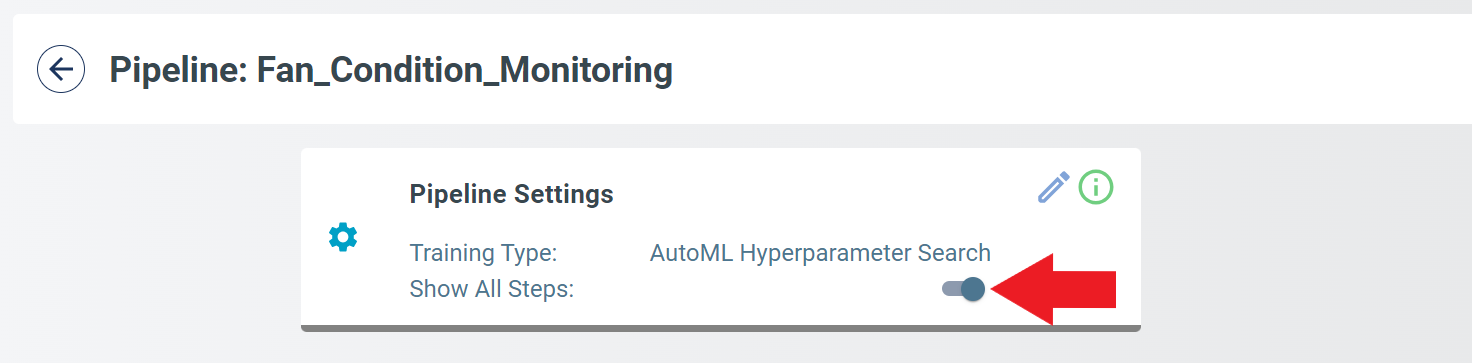
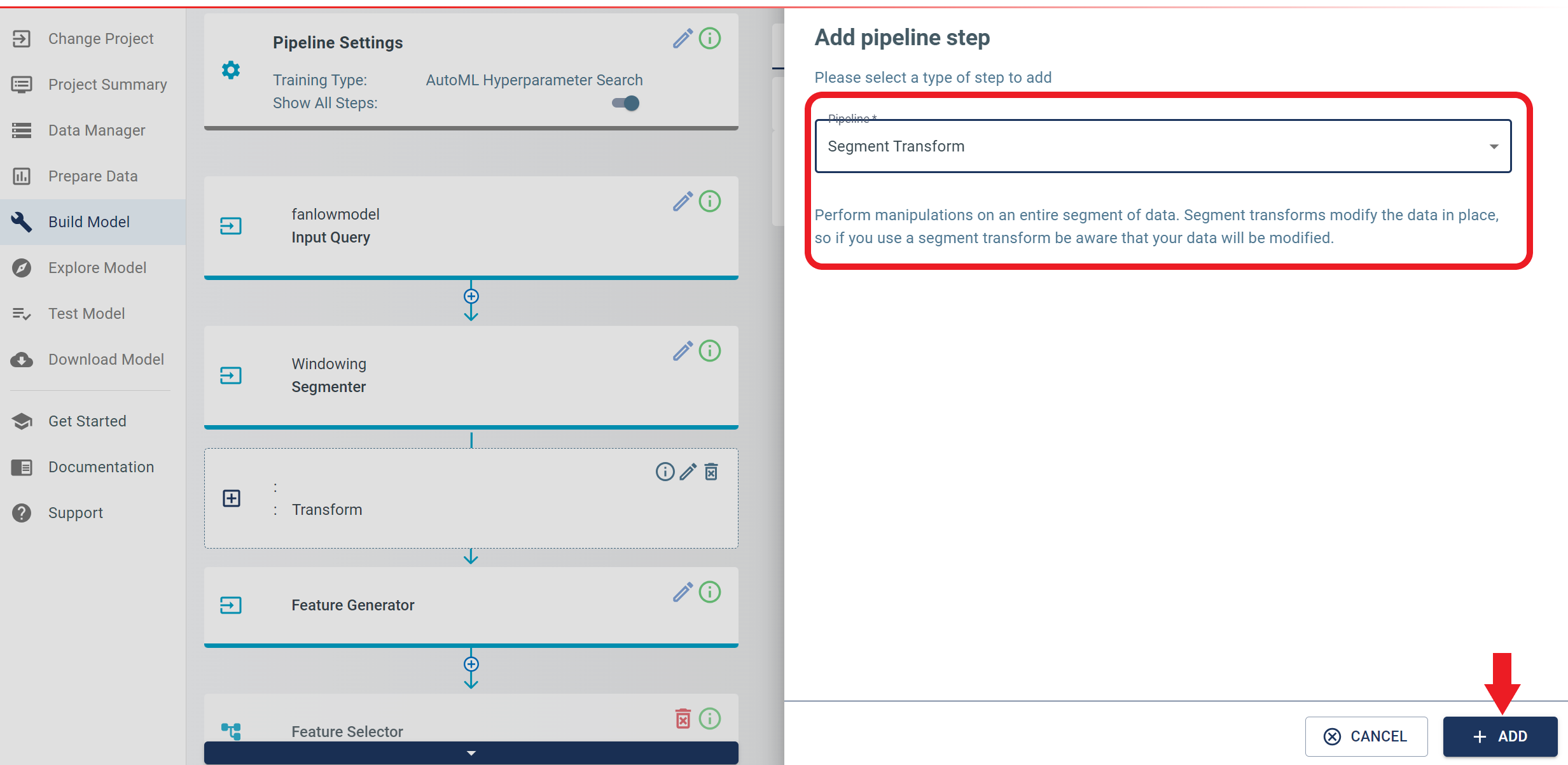
The Pipeline will have all the basic settings configured until here. Next, enable the “Show All Steps” toggle, so that some additional advanced features can be changed.
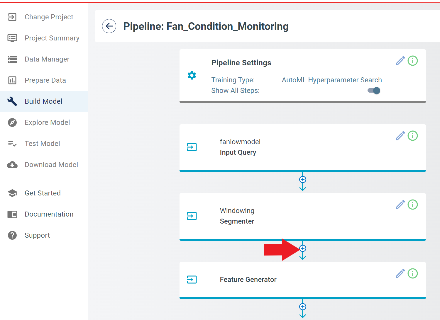
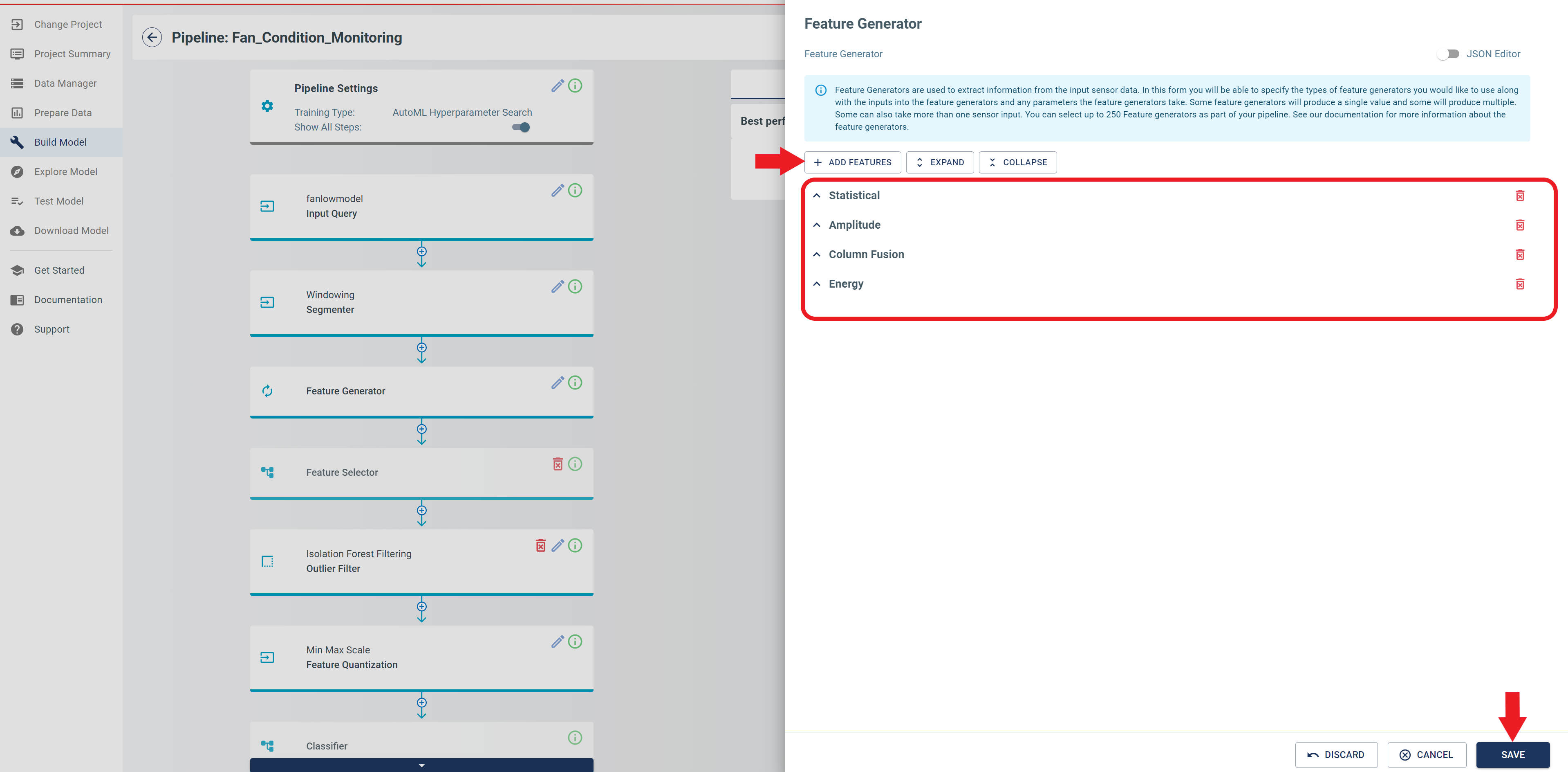
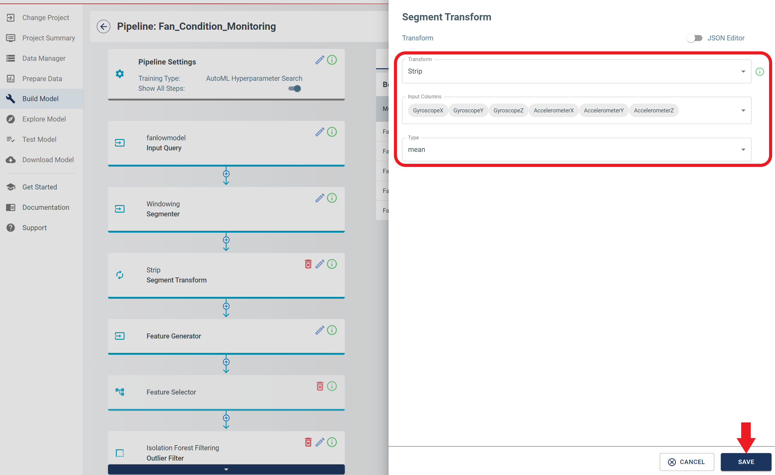
In the Add pipeline step, select Segment Transform from the “Pipeline” drop-down, then click add.
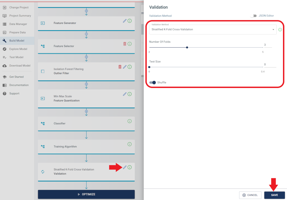
Lastly, click the Validation tab. This is a validation scheme that splits the data set into training, validation and (optionally) test sets based on the parameters. Select the appropriate validation method based on the project requirements. When the validation method is chosen, specify the “Validation Method”, the “Number Of Folds” and the “Test Size” to be used for the validation process. After providing these inputs, click the SAVE button to save the changes made to the validation module.
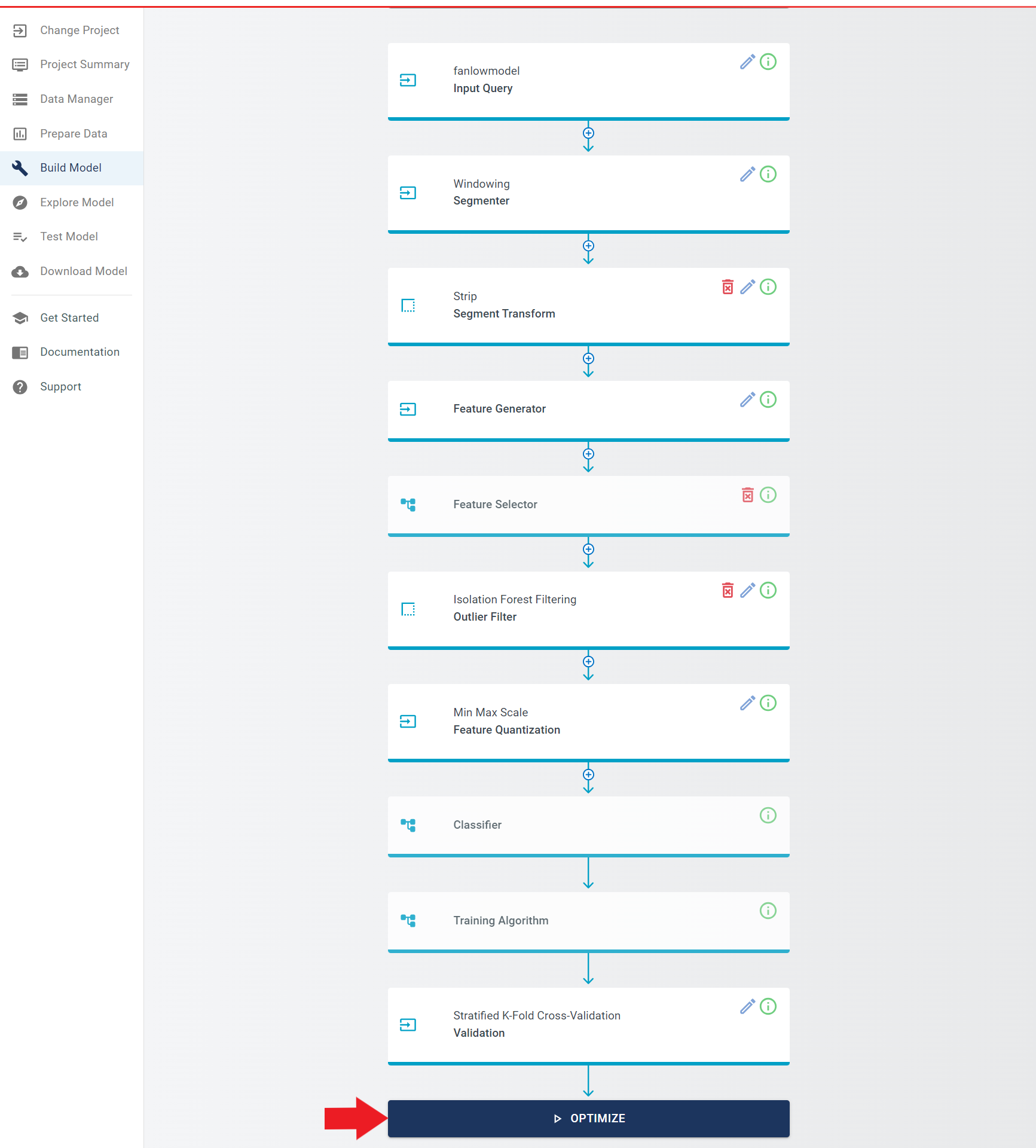
Finally, click the OPTIMIZE button to start the model building process.
After the completion of the Build Model optimization step, proceed to the Test Model view by navigating to it.
To filter the data and select only the test samples, follow these steps:
- Select the Session you wish to work with.
- Locate the upside-down triangle icon in the Fold column, then click it.
- From the drop-down menu, select Test to filter the data and display only the test samples.
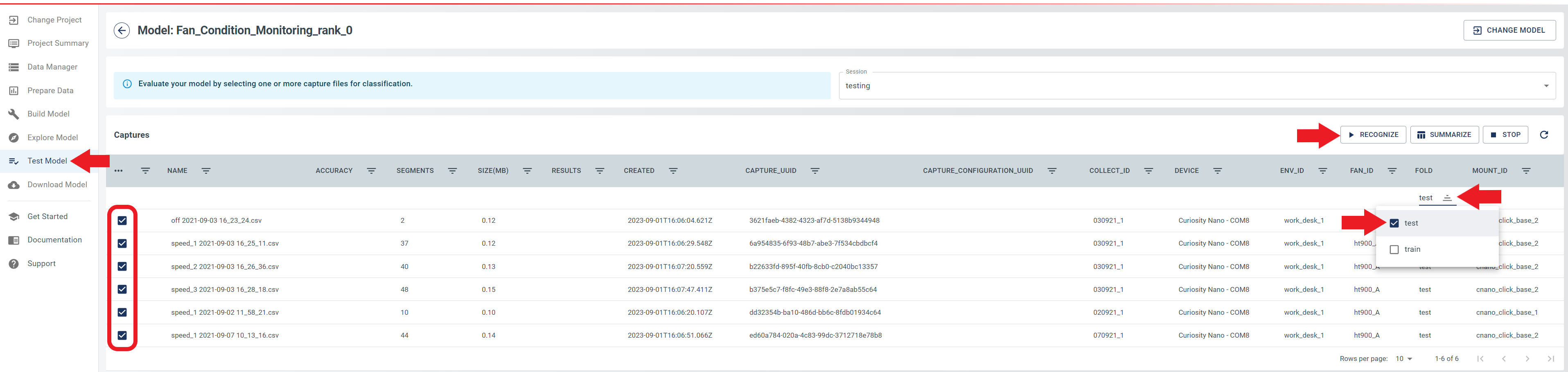
- Locate the ellipsis (…) icon located at the left-most column of the table, then click it.
- From the drop-down menu, select Select All to include all test samples in the analysis.
- Click the Recognize button to begin computing accuracy metrics for the selected samples.
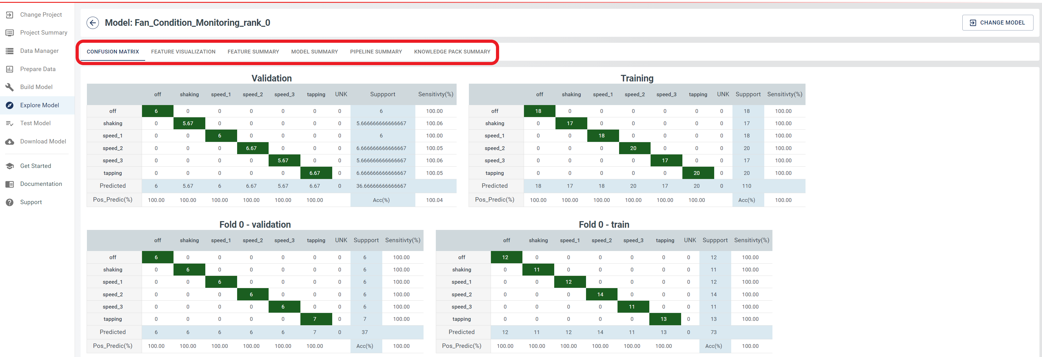
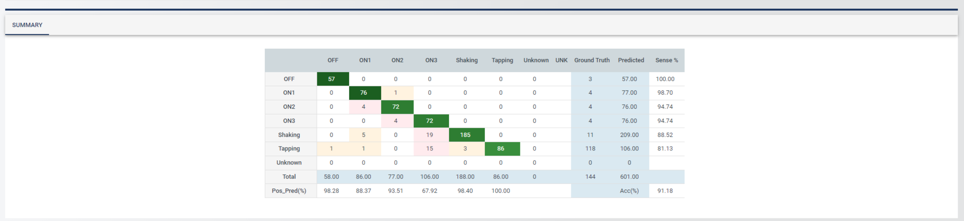
- When the accuracy is computed, click the Summarize button to generate the confusion matrix for the test samples.
- Note that this process may take a few minutes to complete. When finished, you will be presented with a table summarizing the classification results.
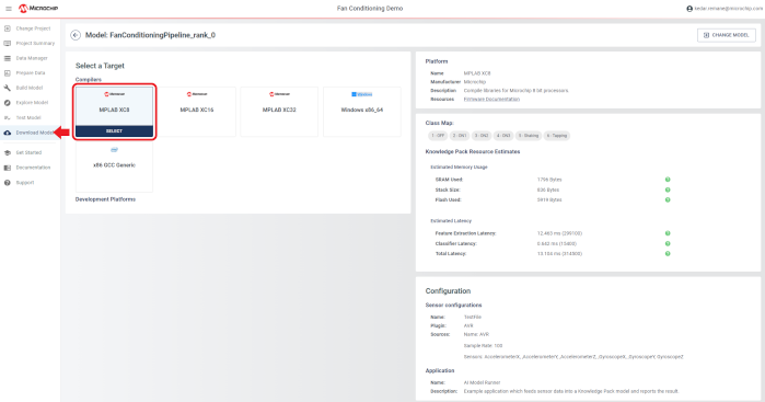
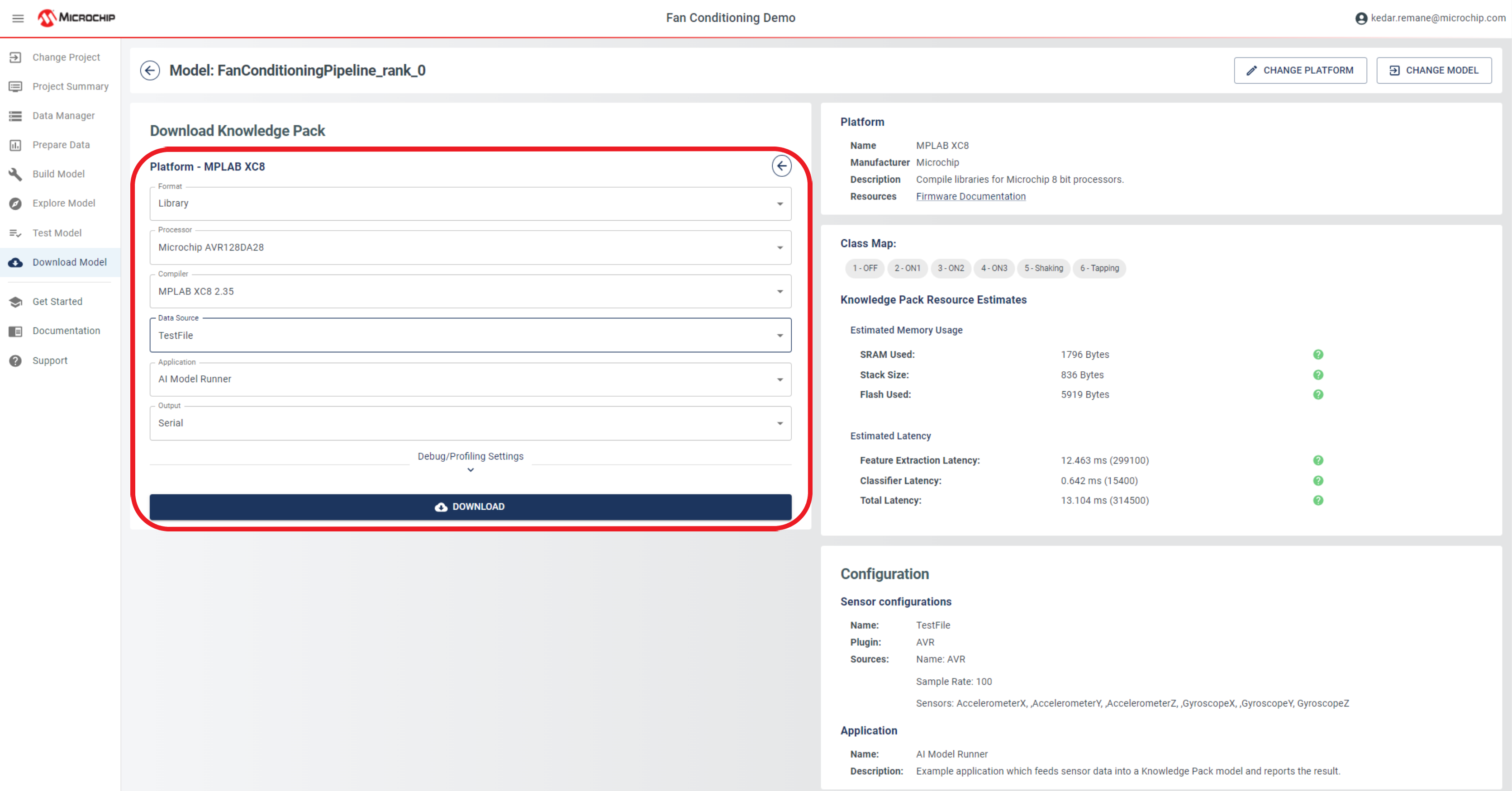
To deploy your model, follow these steps:
- Navigate to the Download Model view.
- Fill out the Knowledge Pack settings using the Pipeline, Model and Data Source you created in the previous steps.
- Select the library output format.
- Click the Download button.
By completing these steps, you will be able to deploy your model and make it available for use. It is important to ensure that all necessary settings are correctly entered before proceeding with the download.
Knowledge Pack Integration
Integrate the Knowledge Pack APIs into your embedded device firmware by following the Knowledge Pack Integration.
Fan Condition Monitor Firmware Overview
For a description of the demo firmware included with this project including operation, usage and benchmarks, see the README file in the GitHub Repository.
Final Remarks
That’s it! You now have a basic understanding of how to develop a Fan State Condition Monitoring application with MPLAB® Machine Learning Development Suite and the AVR DA evaluation kit. For more information about Machine learning at Microchip, visit Artificial Learning and Machine Learning.