4.2 Use Case 2 Output Filter Computation

In Use Case 2: Stereo Class D Amplifier with External Single-Ended Power Stage, the single output of the power stage defaults to a 50% duty cycle square wave, which is pulse-width-modulated to transmit the audio signal in the baseband. Both the DC component (Vsupply/2 on average) and the carrier must be suppressed to protect the speaker, the former through a DC blocking serial capacitor C_s, and the latter by an L-C smoothing filter. This can be simulated with Mindi™ using the 8Ohms 20Hz-20kHz maximally flat SE output filter.wxsch file, available from the MPLAB® Mindi™ Analog Simulator Software Library. See the Appendix.

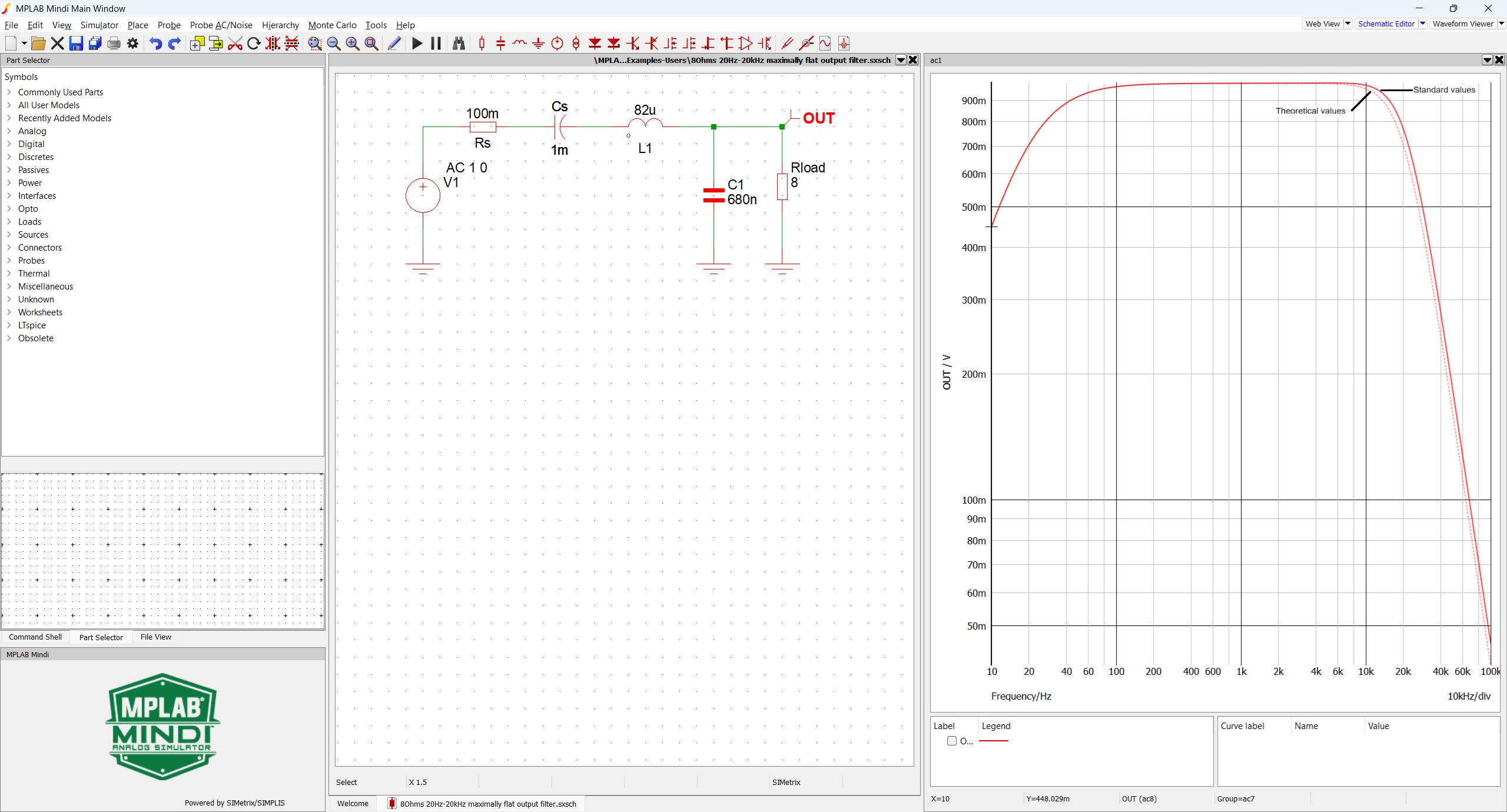
Figure 4-5. Single-Ended Case Passive Smoothing Filter

C_s combines with R(load) to create the first-order high-pass transfer function:
T_HP(s)=RC_s s/(1 + RC_s s)
When fitted to the generic first-order high-pass filter frequency response T(s)=(s/ω_c)/(1+s/ω_c), the selection is:
C=1/(R ω_c), with ω_c=2π f_HP
L1 and C1 combine with R(load) to create the T(s)=1/(1+L/R s + LC s²) low-pass transfer function.
When fitted to the generic second-order low-pass filter frequency response T(s)=1/(1+1/Q*(s/ω_c)+(s/ω_c)²), the selection is:
L=R/(Q ω_c) and C=Q/(R ω_c), with ω_c=2π f_LP

For example, L and C can be computed as functions of R for f_HP=20 Hz, f_LP=20 kHz and Q=1/√2 (Butterworth). See the following table.

Table 4-1. Single-Ended Case Passive Smoothing Filter Components vs Load
R (Ω)	Cs (µF)	L (µH)	C (µF)
1	7958	11	5.63
2	3979	23	2.81
4	1989	45	1.41
8	995	90	0.70
16	497	180	0.35
32	249	360	0.18
64	124	720	0.09
128	62	1441	0.04

If the load is not well defined (as is often the case), a compromise must be found. A high sampling frequency allows relaxation of the cut-off frequency to gain a degree of freedom, but the Q factor must be kept within a suitable range. The table below illustrates how the Q factor influences the shape of the frequency response.

Table 4-2. Effect of Q Factor on Frequency Response Shape¹
Q	G(Flp) [dB]	G(Flp) vs Maximally Flat Filter [dB]	Fr/Flp	G(Fr) [dB]
0.2	-14.0	-11.0	N/A	N/A
0.3	-10.5	-7.5	N/A	N/A
0.4	-8.0	-5.0	N/A	N/A
0.5	-6.0	-3.0	N/A	N/A
0.6	-4.4	-1.4	N/A	N/A
0.707	-3.0	0.0	N/A	N/A
0.8	-1.9	1.1	0.47	0.2
0.9	-0.9	2.1	0.62	0.7
1	0.0	3.0	0.71	1.2
1.1	0.8	3.8	0.77	1.8
1.2	1.6	4.6	0.81	2.4
1.3	2.3	5.3	0.84	3.0
1.4	2.9	5.9	0.86	3.5
1.5	3.5	6.5	0.88	4.0

Note:

Flp is the filter corner frequency; Fr is the resonance frequency for Q>1/√2.

Compared to a system with the same Flp and Q=1/√2, listeners are unlikely to notice any effect on frequency response flatness until Q falls outside the [0.5, 1] range. When Q is in the [0.35, 0.5] range, the loss in high frequencies may become more noticeable, but it remains acceptable. If Q exceeds 1, listeners are likely to quickly perceive harshness and/or sibilance.