
4.3 Use Case 3 Output Filter Computation
A fourth-order filter is typically built from two second-order filters, using Q1 and Q2 as quality factors. A good approximation can be achieved using Q’1 and Q’2 with Q’1*Q’2=Q1*Q2. When using a single amplifier, the only quality factor under control is Q’2, while the two passive RC cells combine into a Q=0.5 second-order cell. Hence, to match a known filter defined by Q1 and Q2, Q=Q1*Q2/0.5 must be used.
As an example, we will refer to the latter case and generate a quasi-B4 filter. A fourth-order Butterworth filter is defined by:
Q1=1/√(2-√2) and Q2=1/√(2+√2)
Q1*Q2=1/√((2-√2)*(2+√2))=1/√(2²-(√2)²)=1/√(4-2)=1/√2
Therefore, Q=√2 (Q=2/√2) must be selected for a single operational amplifier.
In Use Case 3: Stereo Audio DAC with Active Differential to Single-Ended Low-Pass Filter, the resulting gain is too high, causing saturation. The gain can be adjusted using the filter calculator as shown below.
The filter calculator (Excel spreadsheet) is available in the MPLAB® Mindi™ Analog Simulator Software Library, together with the simulation bench (file Datasheet_differential_active_filter_corrected.wxsch). See the Appendix.
| Parameters | Value | Unit | Warnings/Suggested Normalized Values | ||||
|---|---|---|---|---|---|---|---|
| Step 1 | Inputs | Fc = | 20000 | Hz |
WARNING: Q>0.5 generates a peak in the step response that must be taken into account in the maximum gain computation to avoid saturating the amplifier output. Reduce the global gain according to the step overshoot and check the transient simulation results. WARNING: Q>1 generates a gain peak at resonance that must be taken into account to avoid saturating the amplifier output. Reduce global gain according to the gain at resonance frequency and check AC simulation results. Do not cumulate step overshoot and extra gain at resonance frequency correction: apply the highest values from both. | ||
| Q = | 1.41 | – | |||||
| INmin = | -3.3 | V | |||||
| INmax = | 3.3 | V | |||||
| OUTmin = | 0.05 | V | |||||
| OUTmax = | 4.95 | V | |||||
| V1 = | 5 | V | |||||
| Capacitors series = | 12 | – | |||||
| Resistors series = | 96 | – | |||||
| Outputs | No sat. |G| max = | 0.74 | – | ||||
| Resonance freq = | 15824 | Hz | |||||
| Extra gain @Fr = | 1.17 | – | |||||
| Step overshoot = | 1.18 | – | |||||
| Min(C2/C1) = | 13.94 | – | |||||
| Suggested C1 = | 1.20E-10 | F | |||||
| Suggested C2 = | 1.80E-09 | F | |||||
| Step 2 | Inputs | Select |G| = | 0.6 | – | |||
| Select R7 = | 1.00E+05 | Ω | |||||
| Select R8 = | 2.20E+04 | Ω | |||||
| Select C1 = | 2.20E-10 | F | |||||
| Select C2 = | 3.30E-09 | F | |||||
| Select C6 = | 6.80E-09 | F | |||||
| Outputs | Min(C2/C1) = | 12.80 | – | ||||
| Computed R0 = | 7.89E+03 | Ω | Nearest value from R0 in E96 series = | 7870 | Ω | ||
| Computed R1 = | 1.11E+04 | Ω | Nearest value from R1 in E96 series = | 11000 | Ω | ||
| Computed R2 = | 1.05E+04 | Ω | Nearest value from R2 in E96 series = | 10500 | Ω | ||
| Computed R3 = | 2.63E+03 | Ω | Nearest value from R3 in E96 series = | 2610 | Ω | ||
| Computed R4 = | 5.00E+04 | Ω | Nearest value from R3 in E96 series = | 49900 | Ω | ||
| Computed R5 = | 5.00E+04 | Ω | Nearest value from R3 in E96 series = | 49900 | Ω | ||
| Computed R6 = | 1.17E+03 | Ω | Nearest value from R6 in E96 series = | 1180 | Ω | ||
| Computed C3 = | 3.03E-09 | F | Nearest value from C3 in E12 series = | 3.2 | nF | ||
| Computed C4 = | 3.18E-07 | F | Nearest value from C4 in E12 series = | 320 | nF | ||
| Computed C7 = | 8.83E-07 | F | Nearest value from C7 in E12 series = | 830 | nF | ||
| R6 induced loss = | 0.94 | – | Effective overall gain = | -0.56 | – | ||
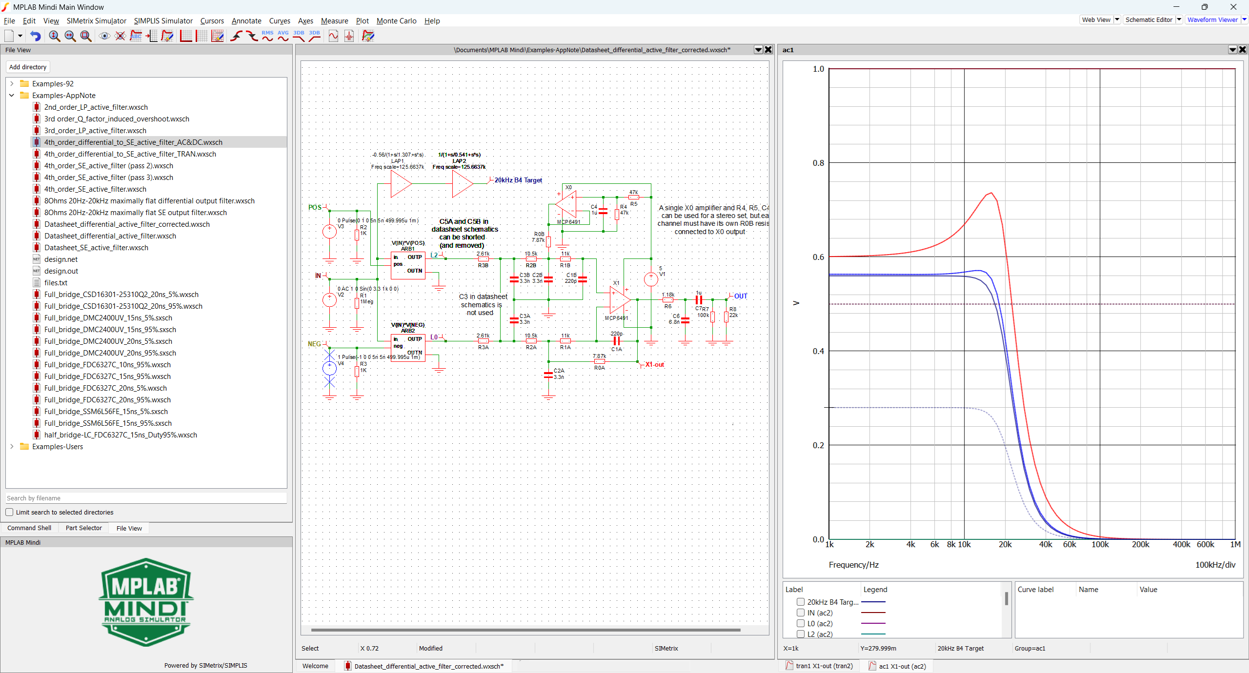
As shown, the response is quite close to the Butterworth target. Some extra damping will help. As mentioned in the filter calculator for the third and fourth orders, the upfront passive first-order cell interferes with the second-order cell. Experience shows that adjusting the C3 value is the best way to bring the behavior back to the target.
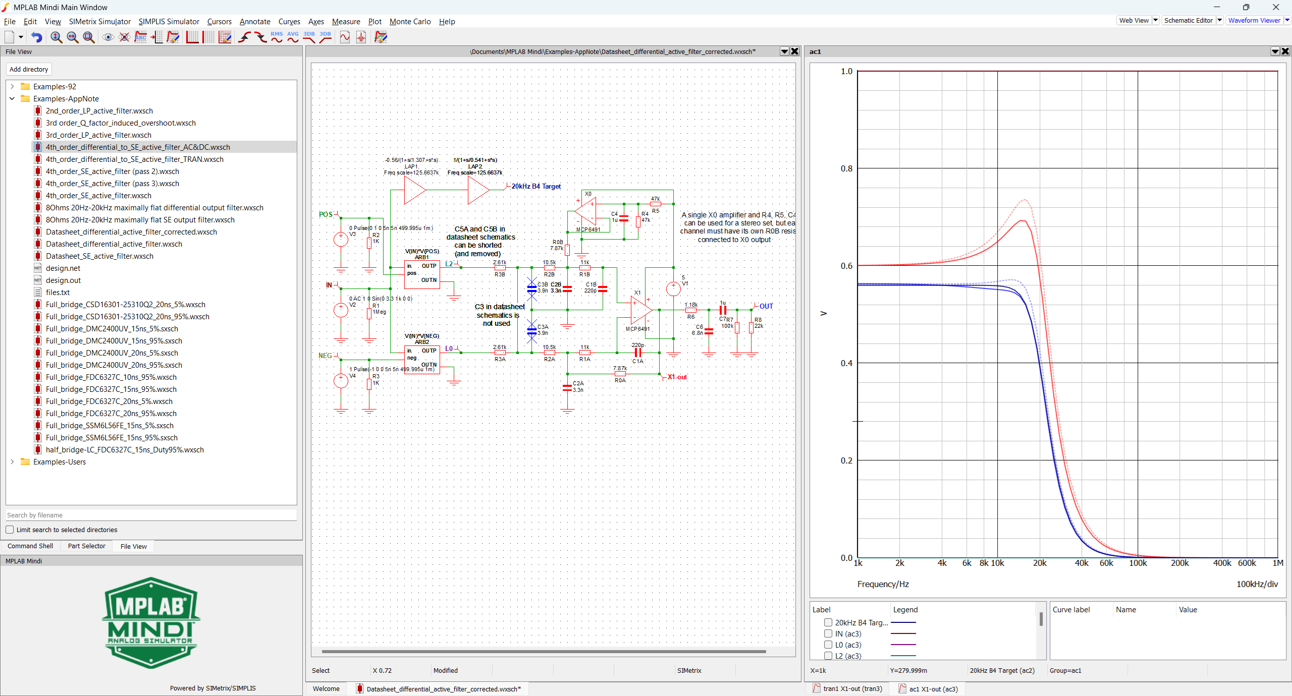
Changing C3 from 3.3 to 3.9 nF brings the simulated response to the B4 target.
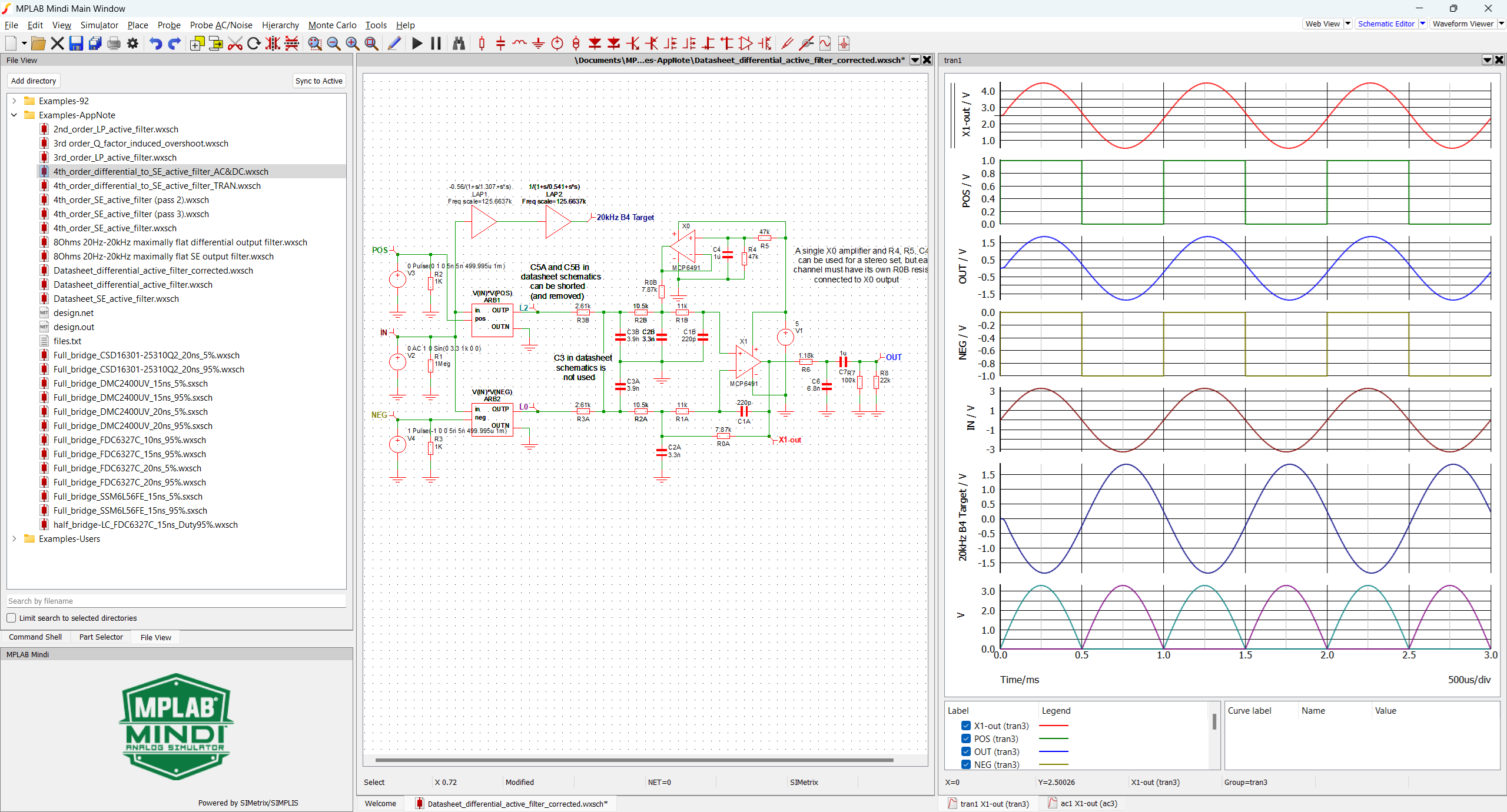
The transient simulation confirms there is no longer any saturation with the full-scale signal.