4.5.1 PC Sampling Example
This section shows PC sampling along with Power Profiling in the same timeplot.
This example is based on an USB MSC example project from Start. We used the SAM L22 Xplained Pro kit, but the procedure is the same for other debuggers and kits that support PC sampling.
Make sure that debugging is started and open the Data Visualizer window.
Find the Debugger Polling interface in the list of DGI interfaces for the connected kit.
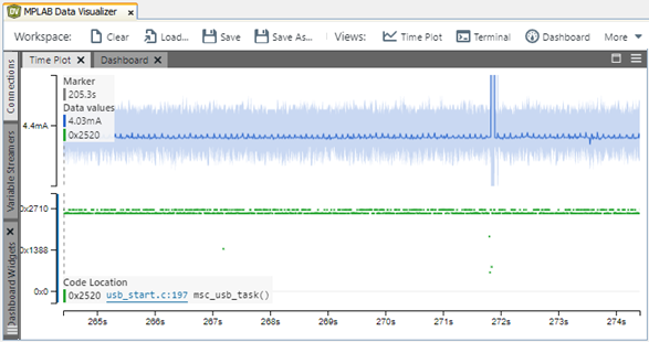
Hover over the interface and plot all sources by clicking  . This will
add the PC Sampling signal to the current timeplot (as shown in the figure below), in
green. The figure also shows a plot of the current consumption, that has already been
added, in blue.
. This will
add the PC Sampling signal to the current timeplot (as shown in the figure below), in
green. The figure also shows a plot of the current consumption, that has already been
added, in blue.
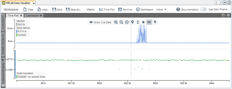
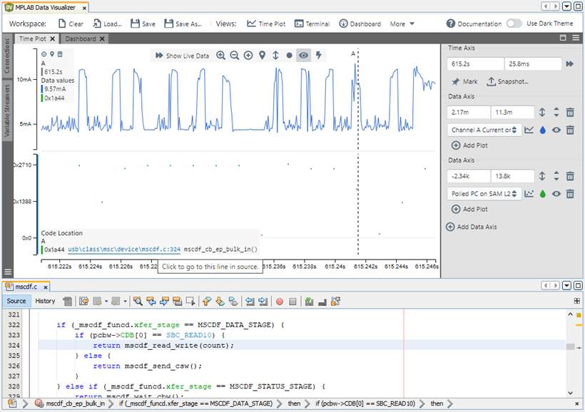
Zoom in on the area of the timeplot that shows the increased power consumption.
Make sure the "Inspect"  function is enabled. When a PC Sampling signal is being
plotted, the PC value that is closest to the cursor will be shown in the inspect values
panel at the left of the plot area. The source code location will be decoded (if
possible) and shown in the lower part of the plot area. In this example a location with
PC value equal to 0x1A44 is being decoded to a function related to the USB MSC
handling.
function is enabled. When a PC Sampling signal is being
plotted, the PC value that is closest to the cursor will be shown in the inspect values
panel at the left of the plot area. The source code location will be decoded (if
possible) and shown in the lower part of the plot area. In this example a location with
PC value equal to 0x1A44 is being decoded to a function related to the USB MSC
handling.
By clicking on the source code link, the file will be opened with the cursor located on the corresponding source line.