4.5.4.2 DC Signal With Random Noise

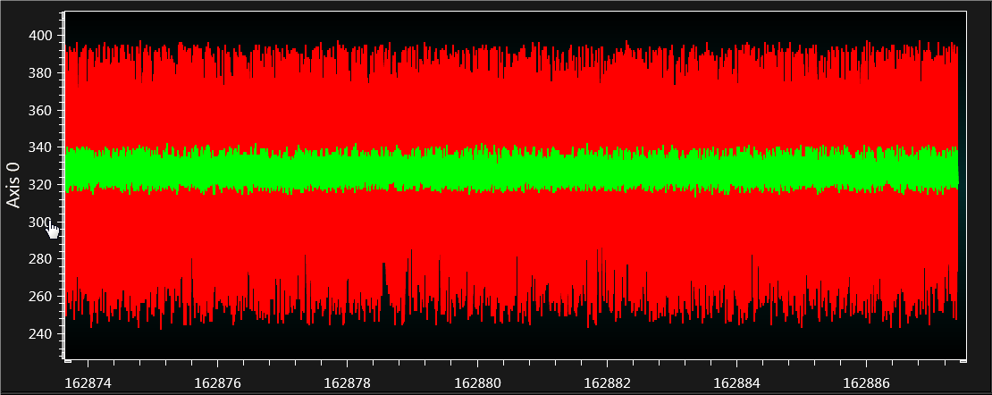
The Data Visualizer graph is as shown in Figure 4-16. The red colored signal is a noisy input signal (ADRES value), the green colored signal is the filtered signal (ADFLTR value).

From the graph, it can be seen that the noise has been suppressed using ADC² Burst Average mode. In example source code averaging has been done with 32 samples as ADCRS bits configured to 5. The graph looks almost similar to the graph for Basic mode, Accumulate mode, and the Average mode where the ADC count of filtered signal (green colored signal) can be seen as ~ 315 to 340.

In Burst Average mode, the ADC count may vary more randomly than in other modes. Here the samples are accumulated in a burst. This means that once the conversion is triggered ADC samples are continuously read until 32 samples are collected. Because of this the noise filtering may not be as effective as other modes.

Use case: This mode can be useful in application where the input signal is relatively noise free and ADC resolution needs to be increased by oversampling.

Pros: Using this mode, the ADACC register gives accumulated values of up to 64 samples and the ADFLTR register gives an average value of all the accumulated samples in a single burst. Software overhead can be avoided.