3.5.1.23.3 Logic Level Distribution

The number of levels of logic (or logic levels) in a design is an indication of how much combinatorial logic (e.g. LUTs, carry-chains) there is between registers (Flip-Flops). The more pipelined the design is, the lower the number of logic levels will be and higher frequencies may be achieved. However, more registers will be required. In general, having lower logic levels is a good practice specially when a design needs to run at higher frequencies.

Different algorithm implementations, HLS #pragmas or even project settings will impact the number of logic levels differently. A logic level distribution plot can help you visualize the impact of those options and assess any tradeoffs. Considering the number of levels of logic early in the design flow allows easier modifications upfront rather than in later stages of the design during the more time-consuming place & route and timing closure processes.

The logic level distribution histogram can easily be generated from the IDE by clicking on SmartHLS -> Plot Logic Level Distribution; or from the command-line by just typing this:

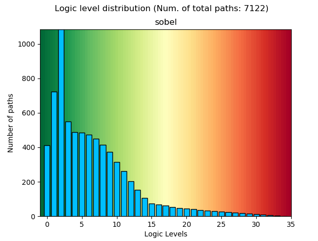
shls logic_level_histogram

This command will run RTL synthesis first, which is required before generating the logic level histogram. After synthesis this command will generate a timing analysis report from which the logic levels are extracted. As an example, for Part1 of the SmartHLS Sobel Tutorial the histogram looks like this:

Two files are generated under the hls_output/reports/ directory:

• logic_level_hist.ta.hist - it is a plain text file that contains the raw histogram data. First column is the logic level, the second column is the number of paths in that level.
• logic_level_hist.ta.png - the plot file in .png format.

The plot shows a gradient from green (left) to red (right) indicating that it would be better for Place & Route and timing purposes to have as many paths towards the left much as possible and minimize those with higher logic levels.