
Visualizing the profiled data
(Ask a Question)Finally, the third step in the profiling process is to parse the generated .prof files and visualize them. This can be done from the IDE by clicking on ; or from the command-line, simply type:
shls
            soc_profiler_view
hls_output/reports/hls_soc_profiler.summary.rpt.Project: soc_profiler --------------------------------- Statistics (units in [us]): --------[ main ]-------- main start : 0.19 us main finish : 11747.38 us main Delta Time : 11747.19 us --------[ hw_const_add ]-------- Number of samples: 10 +-------------+-------+--------+-------+-----------+ | | min | max | avg | aggregate | +-------------+-------+--------+-------+-----------+ | Write | 50.76 | 208.28 | 69.08 | 690.76 | | Accelerator | 5.42 | 6.62 | 5.59 | 55.94 | | Total | | | | 746.7 | +-------------+-------+--------+-------+-----------+ --------[ hw_const_mult ]-------- Number of samples: 10 +-------------+------+-------+-------+-----------+ | | min | max | avg | aggregate | +-------------+------+-------+-------+-----------+ | Write | 3.82 | 7.74 | 4.3 | 42.98 | | Accelerator | 4.74 | 4.83 | 4.77 | 47.7 | | Read | 40.3 | 52.18 | 47.31 | 473.1 | | Total | | | | 563.78 | +-------------+------+-------+-------+-----------+ --------[ hw_delay ]-------- Number of samples: 100 +-------------+------+---------+------+-----------+ | | min | max | avg | aggregate | +-------------+------+---------+------+-----------+ | Write | 0.44 | 3.25 | 0.48 | 48.36 | | Accelerator | 2.7 | 2000.96 | 22.7 | 2270.25 | | Read | 0.46 | 0.88 | 0.47 | 47.03 | | Total | | | | 2365.64 | +-------------+------+---------+------+-----------+ --------[ hw_sum ]-------- Number of samples: 10 +-------------+-------+-------+-------+-----------+ | | min | max | avg | aggregate | +-------------+-------+-------+-------+-----------+ | Write | 3.62 | 6.79 | 4.09 | 40.88 | | Accelerator | 23.12 | 23.71 | 23.21 | 232.11 | | Read | 0.46 | 0.68 | 0.48 | 4.81 | | Total | | | | 277.8 | +-------------+-------+-------+-------+-----------+
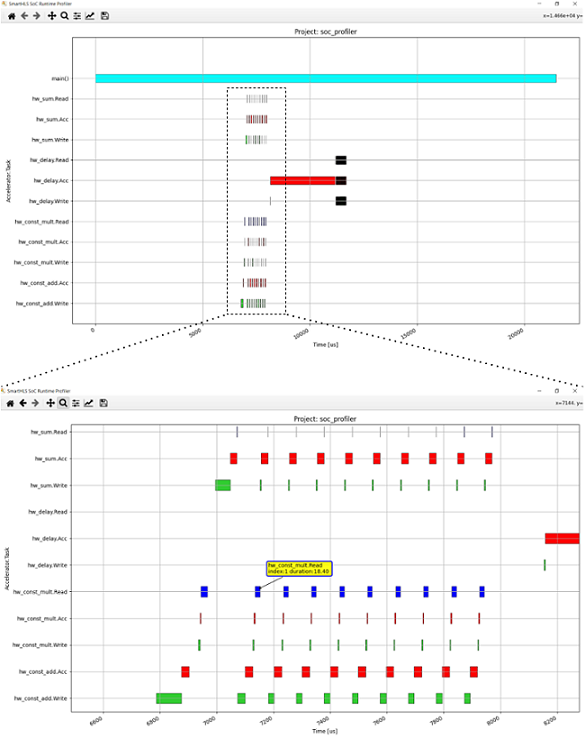
In this context, the word Write refers to the time that the CPU spent
writing data to the hardware module. The word Accelerator (or
Acc in the plot below) refers to the time the hardware module was
active. And finally, the word Read refers to the time that the CPU spent
reading data from the hardware module's on-chip buffers. The command shls
soc_profiler_view will also open up a GUI that shows a plot of the runtime. The
GUI has a way to zoom-in to specific region of the plot. Also, the mouse pointer can hover
over specific bar on the plot and the corresponding annotated data will be displayed.
By default, the plot will display the timelines for all the hardware modules in the project
by including all the *.prof files in the plot. However, a single timeline for a
specific hardware module can be displayed using the SOC_PROFILER_FILENAME makefile
variable and assign to it the specific .prof file to visualize. For example, to
display only the time line for the hardware module hw_const_sum() you can
type this:
shls soc_profiler_view SOC_PROFILER_FILENAME=./hls_output/files/hls_hw_const_sum.prof
Note the hls_ prefix in the filename. The plot will look like this:

In some cases, such as in automated regression tests, an interactive GUI is not required or not even desired. The profiler can be run in non-interactive mode like this:
shls soc_profiler_view SOC_PROFILER_INTERACTIVE=0
In this case the summary file is still generated and printed to the terminal but the GUI
plot will not be displayed. Instead an image file with .png format will be generated
under hls_output/reports/hls_soc_profiler.png. Note that this
non-interactive option is only available from the command-line.
At the moment, the SoC Profiler only measures the time for arguments declared as
AXI Target, with or without DMA. Arguments defined as AXI
Initiator will only show a small bar in the write timeline
representing the CPU passing the pointer address from which the hardware module will
initiate read or write requests. The AXI Initiator transfer time is
implicitly considered as part of the hardware module runtime (i.e. Acc timeline).
In the example above, the hw_const_add() module has no read time. That is
because the CPU is not reading the on-chip buffer, the hardware module itself is
transferring the data back to the CPU memory directly and therefore the time consumed is
considered as part of the module execution runtime.